1. Introduction
ireless Sensor Networks (WSNs) consist of many no of small nodes .It can be an effective for collecting data from various environments. Each sensor sends its data to Base Station (BS) [4], and finally BS sends these data to end user. Clustering is considered as an effective approach to provide better data gathering and scalability for large sensor networks.
Sensor networks are the combination of distributed sensing, communication and computing. also required in order to accurately estimate the target in a sensor field.
2. II.
3. Literature Survey
A wireless sensor network is an autonomous system of numerous tiny sensor nodes equipped with integrated sensing and data processing capabilities. These sensor networks are distinguished from other wireless networks by the fundamental constraints under which they operate, i.e., sensors have limited and unreplenish able power resources making energy management a critical issue in wireless sensor networks. So these sensors must utilize their energy as efficiently as possible.
Many no of sensors are randomly placed and the target does not follow a single uniform path. So the main challenge is to track the moving target .So it requires an efficient navigation control method. Enyang and Soura [1] studied a set of different algorithm for node deployment like TOA algorithm. Generally a target is signal emitter whose transmission is received by a number of sensors that is placed distributedly. Distributed inference methods [8] developed for graphical models comprise a principled approach for data fusion in sensor networks. The application of these methods, are distributed nature of computation and deployment coupled with communications bandwidth and energy constraints typical of many sensor networks. Traditional measures [1] of distortion are not sufficient to characterize the quality of approximation as they do not address in an explicit manner the resulting impact on inference .While both graphical models and a distributed sensor network [8] have network structures associated with them.
4. III.
5. New Contributions
We are interested in target tracking by considering both moving targets and mobile sensors. The spatial resolution refers to how accurate a target's position can be measured by sensors, and the actual paths in wireless sensor networks. Here we used Time To Live (TTL) for route discovery and also we considered Min Hop for finding the path .We define the spatial resolution as the deviation between the estimated and the actual target trajectory path, which can be explained as the distance that a target is not covered by any mobile sensors. It includes a more general TOA [8] measurement model that accounts for the measurement noise due to multipath propagation and sensing error.
6. IV.
7. Problem Statement
The problem of tracking signal-emitting mobile targets using navigated mobile sensors based on signal reception. The Mobile Sensor Collection node will initiate communication with other sensor nodes in the network and finds multiple measurements with respect to the target location and then the time of arrival of each signal from the sensor nodes is computed with respect to target by the mobile sensor collector node. The path which has the lowest TOA is said to be trajectory of the mobile node in the network. But this project not only computes the TOA [8] but only measures the spatial separation with respect to degrees so that the TDD [5] of the mobile target is also captured. The node deployment algorithm, which is responsible for deploying the nodes in a sensor area consider TTL and mean hop. It also checks which nodes are within the coverage range and which are not. The target is tracked by angular position discovery algorithm.
V. Consider a uniform linear array geometry with L elements numbered 0, 1,?, L-1 with a spacing of have half wavelength spacing ( ) between them. Let be the baseband signal that is received by each array element, but at a different time instant. If the phase of baseband signal received at element 0 is zero. By examining the geometry from figure 1, using basic trigonometry and facts from wave propagation, the time delay of arrival can be computed as
8. Mathematical Modeling
Where, is the speed of light, is an integer and is the direction from which plane wave is impinging on Sensor array Suppose is a narrowband digitally modulated signal with low pass equivalent, carrier frequency , and symbol period . Narrow band signal can be written as
{ } t f j l c e t b t b ? 2 ) ( Re ) ( = (2)The signal received by the k th element is given by ( )
) ( 2 ) ( Re ) ( k c t t f j k l k e t t b t x ? ? ? ? = ? (3)Now suppose that the received signal at the k th element is down converted to the baseband. In that case, the baseband received signal is defined as
k c t f j k l k e t t b t x ? ? ? ? = ? 2 ) ( ) ((4)VI.
9. Methodology 1. Node Deployment
This is responsible for placing the nodes in a given area
10. Coverage Area Determination
This module is used to determine the nodes which are reachable or to which a given sensor node can communicate directly 3. Picking the Next Sensor
The next sensor is picked randomly and target location is determined with respect to given sensor area.
11. Measuring the TOA
The TOA is measured with respect to the distance of the node and time of arrival of the detection packets.
12. Measuring the TDD
The Target Direction Detection of the signals with respect to the target is measured using MEV and CRLB approach VII.
13. Tracking Algorithms a) Node deployment algorithm
The Node Deployment algorithm is used to randomly disperse the nodes across the network. It will place the node randomly in a network. Then TTL=TTL-1
The Individual Route Discovery Module is implemented by Time of Arrival 2 algorithm. . When a source node wants to send data to the sink, it includes a TTL of initial value N. It then randomly selects a neighbor for each share, and uni-casts the share to that neighbor. After getting the share, the neighbor first decrements the TTL. If the new TTL is greater than 0, then compares the neighbor list obtained from routing table with the list of nodes present in Node in Route (NIR Field). After getting the set of nodes not present in NIR. The neighbor is randomly picked from the neighboring nodes .When the TTL becomes 0, the last node receiving that share stops the random propagation of this share, and starts mooving it toward the sink using normal min-hop routing. The Min-Hop Routing algorithm picks the farthest node of its transmission range.
The minimum Hop Routing Algorithm used in the algorithm when TTL becomes zero works as below Min Hop routing algorithm picks the neighbor which is closest to the destination node. i.e. farthest node which is reachable.
14. c) Target Direction Detection Algorithm
Target Direction Detection of a mobile node with respect to spatial separation using different Filters approach are as follow. We can get from (4) The received baseband signal after sampling with a sampling period of T seconds is given by
K c t f j K l k e t T n b nT x ? ? ? ? = ? 2 ) ( ) ((5)In a wireless digital communication system, the symbol period will be much greater than each of the propagation delays across the array given by
1 ,......., 1 , 0 , ? = ? L k t T K ?? (6)This allows the following approximation to be made
K c t f j l k e nT b nT x ? ? ? ? 2 ) ( ) ((7)The constants c and c f can be related through the basic equation
? c f c = (8)Where, ? is the wavelength of the propagating wave and c f is the carrier frequency. The element spacing can be computed in wavelengths by using
? D d = (9)Using the equations ( 1) and ( 8) in equation (7) we can arrive at equation
c kD c j l t f j l k e nT b e nT b nT x K c ) sin( 2 2 ) ( ) ( ) ( ? ? ? ? ? ? ? = ? (10)Substituting the value of 'D' from equation (9) in equation (10) gives
c d k c j l k e nT b nT x ) sin( 2 ) ( ) ( ? ? ? ? ? ? (11)After simplifying, we get
) ( sin 2 ) ( ) ( ? ? d k j l k e nT b nT x ? ? (12)When discrete time notation is used with time index n, equation ( 12) can be written as
) ( ) ( ) ( ) ( ) ( sin 2 ? ? ? K d k j k a n b e n b n x ? ? ? (13)Let the n th sample of the baseband signal at the k th element be denoted as
) (n x k.When there are M signals present, the n th symbol of the i th signal will be denoted by
) (n b i for 1 ,...., 2 , 1 , 0 ? = M i. The baseband sampled signal at the k th element can be expressed as
) ( ) ( ) ( 1 0 i M i i k a n b n x ? ? ? = ? (14) i.15. Formulation of Array Data Matrix
By considering all the array elements, i.e
? ? ? ? ? ? ? ? ? ? ? ? ? ? ? ? ? ? ? ? + ? ? ? ? ? ? ? ? ? ? ? ? ? ? ? ? ? ? ? ? ? ? ? ? ? ? ? ? ? ? ? ? ? ? ? ? ? ? ? ? = ? ? ? ? ? ? ? ? ? ? ? ? ? ? ? ? ? ? ? ? ? ? ? ? ? ? ? ? ? 1 1 0 1 1 0 1 1 1 1 0 1 1 1 1 1 0 1) ( ) ( 1 1 1 1 0 1 1 1 1 1 0 1 1 0 1 0 0 0 ? ?(17)ii.
n a n V V R ? = (24)Where n V is Lx1 matrix comprising of unknown variables. Expanding equation (24) in matrix notation,
? ? ? ? ? ? ? ? ? ? ? ? ? ? = ? ? ? ? ? ? ? ? ? ? ? ? ? ? ? ? ? ? ? ? ? ? ? ? ? ? L a L L L L L L L V V V V V V R R R R R R R R R ? ? ? ? ? ? ? ? ? 2 1 2 1 , 1 , 0 , , 1 1 , 1 0 , 1 , 0 1 , 0 0 , 0 ? (25)16. Global Journal of Computer Science and Technology
Volume XIV Issue IV Version I
I A R A R H ss 2 ? + = (21)Multiplying the matrices, a set of simultaneous equations as defined in (26) are obtained . These L values form Eigen vector matrix.
L a L L L L L a L L a L L V V R V R V R V V R V R V R V V R V R V R ? ? ? = + + + = + + + = + + + , 2 1 , 1 0 , 2 , 1 2 1 , 1 1 0 , 1 1 , 0 2 1 ,17. a. Kalman Filter
This method finds a power spectrum such that its Fourier transform equals the measured correlation subjected to the constraint that its entropy is maximized. For estimating TDD from the measurements using an array of sensors, the Kalman method finds a continuous function P MEv (?) > 0 such that it maximizes the entropy function. The Kalman power spectrum is given by The Maximum Margin Analyzer is known as a MMA. It is also alternatively a maximum likelihood estimate of the power arriving from one direction while all other sources are considered as interference. Thus the goal is to maximize the Signal to Interference Ratio (SIR) while passing the signal of interest undistorted in phase and amplitude. The source correlation matrix ss R is assumed to be diagonal. This maximized SIR is accomplished with a set of array weights given by
) ( ) ( 1 ? ? a E E a P H s S H KALMAN =() ( ) ( ) ( 1 1 ? ? ? a R a a R w xx H xx mma ? ? = (28)Where,
1 ? xxR is the inverse of un-weighted array correlation matrix xx R and ) (? a is the steering vector for an angle ? . The MMA pseudo spectrum is given by
) ( ) ( 1 ? ? a R a P inv H MMA = (29) c. WMMA FilterIn this method [10] a rectangular window of uniform weighting is applied to the time series data to be analyzed. For bearing estimation problems using an array, this is equivalent to applying equal weighting on each element. WMMA Filter method is also called Ordinary Beam forming Method (OBM). This method estimates the mean power P B (?) by steering the array in ? direction. The power spectrum in WMMA Filter method is given by
2 ) ( L RS S P H WMA ? ? ? = (30)Where, 'S ? ' denotes the steering vector associated ?, 'R' is the array correlation matrix. 'L' is the number of elements in the array In DOA estimation, a set of steering vectors {S?} associated with various direction ? is often referred to as the array manifold. From the array manifold ,the array correlation matrix, PB(?) is computed. Peaks in P B (?) are then taken as the directions of the radiating sources.
18. d. CRLB Filter
CRLB is an acronym which stands for Carmer Roa Bound. CRLB provide correct estimates of the number of signals, angles of arrival and the strengths of the signal. CRLB makes the assumption that the noise in each channel is uncorrelated making the noise correlation matrix diagonal. However, under high Signal correlation the traditional CRLB algorithm breaks down and other methods must be implemented to correct this weakness.
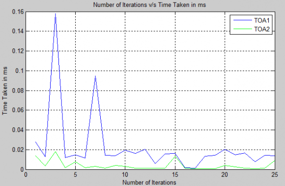
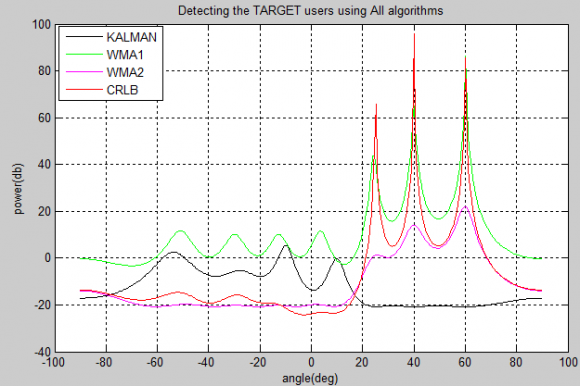
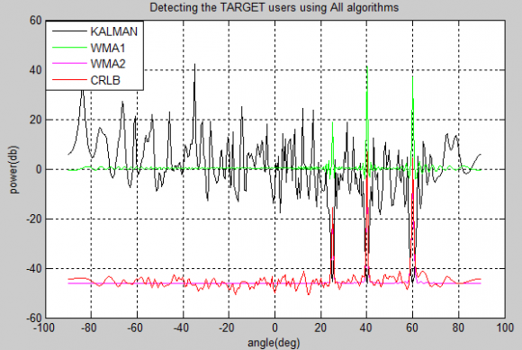
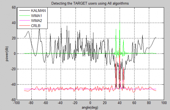
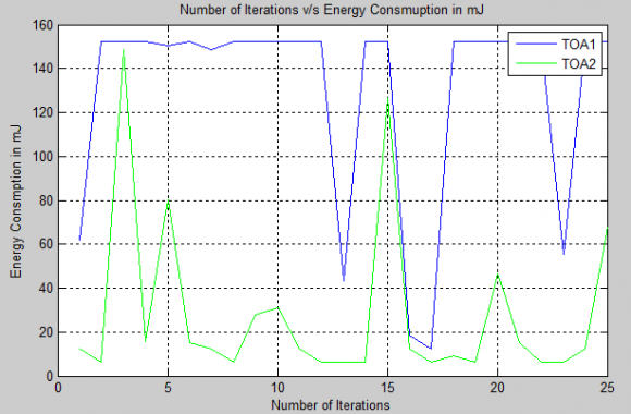
The Eigen values and eigenvectors for correlation matrix R is found. Figure 2 shows route discovery algorithm using TOA, which contains 30 nodes that are randomly placed. The source node is 8 and the target node is 23. From the above table it is clear that the power and energy required for TOA2 algorithm is less than TOA1 algorithm. The second algorithm takes less time as compared to first one and also it takes less no hopes. From the plot it is evident that the CRLB and WMA1 detects all the three targets as shown in the figure 11 where WMA2 also detects targets whereas and Kalman filter is not able to detect all the targets. IX.
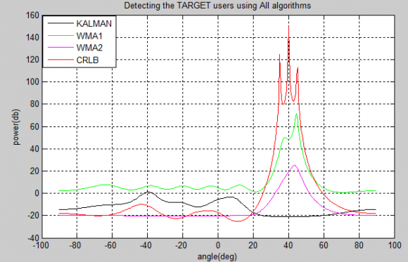
19. d) Comparison Filter Target Detection for Less Sensor Elements and Widely Spaced Sources
20. Conclusion
From the various simulations we can find out that CRLB works best as compared to all other algorithms for various cases like Low Sensors and Widely spaced targets, Low Sensors and Closely Spaced targets, Large Sensors and Widely Spaced targets and finally large sensor and closely spaced sources. From the various simulations one can prove that the TOA2 algorithm works better as compared to TOA1 algorithm with respect to energy, time, power and no of hops.
Algorithms can be future improved by maintaining the route trace list thereby reducing the energy, time, power and number of hops.

![M signals (sources). iii. Finding Eigen value and Eigen Vectors of Array Correlation MatrixEigen values and eigenvectors[4] provide useful and important information about a matrix. It is possible to determine whether a matrix is positive definite, invertible, indicate how sensitive determination of inverse will be to numerical errors. Eigen values and eigenvectors are useful in spectrum estimation and adaptive filtering problems.The Eigen values of LxL Array Correlation matrix R is found by solving the characteristic equation given by for specific Eigen value a ? is found by solving the equation given by](https://computerresearch.org/index.php/computer/article/download/116/version/100846/1-Performance-Evaluation-of-Target_html/14514/image-5.png)

![is the i th Eigen Value.The noise subspace Eigen vectors[4] are orthogonal to the array steering vectors at the angles of arrival M is the inverse of autocorrelation matrix.](https://computerresearch.org/index.php/computer/article/download/116/version/100846/1-Performance-Evaluation-of-Target_html/14517/image-8.png)