1. Introduction
nalysis of texture requires the identification of proper attributes or features that differentiate the textures in the image for segmentation, classification and recognition. Initially, texture analysis was based on the first order or second order statistics of textures [6,7,8,9,10]. Then, Gaussian Markov random field (GMRF) and Gibbs random field models were proposed to characterize textures [11,12,13,14,15,16]. Later, local linear transformations are used to compute texture features [17,18]. Then, texture spectrum technique was proposed for texture analysis [19]. The above traditional statistical approaches to texture analysis, such as co-occurrence matrices, second order statistics, GMRF, local linear transforms and texture spectrum are restricted to the analysis of spatial interactions over relatively small neighborhoods on a single scale. As a consequence, their performance is best for the analysis of micro textures only [20]. More recently, methods based on multi-resolution or multichannel analysis, such as Gabor filters and wavelet transform, have received a lot of attention [21,22,23,24,25,26,27,23,25]. From the literature survey, the present study found the Gray Level Co-occurrence Matrix (GLCM) is a benchmark method for extracting Haralick features (angular second moment, contrast, correlation, variance, inverse difference moment, sum average, sum variance, sum entropy, entropy, difference variance, difference entropy, information measures of correlation and maximal correlation coefficient) or Conners features [28] (inertia, cluster shade, cluster prominence, local homogeneity, energy and entropy). These features have been widely used in the analysis, classification and interpretation of remotely sensed data. Its aim is to characterize the stochastic properties of the spatial distribution of grey levels in an image.
The present paper is organized as follows. In he second section we have given clear information about grey level co-occurrence matrix information and the third section we discussed about textons. In fourth section we discussed deriving different Shape Descriptor Indexes (SDI). In the fifth section, proposed methodology is discussed and in sixth section results and discussions are given. Finally in last section we concluded about this paper.
2. II.
3. Gray Level Co-occurrence Matrix
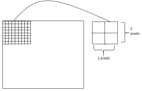
One of the other most popular statistical methods used to measure the textural information of images is the Gray Level Co-occurrence Matrix (GLCM). The GLCM method gives reasonable texture information of an image that can be obtained only from two pixels. Grey level co-occurrence matrices introduced by Haralick [29] attempt to describe texture by statistically sampling how certain grey levels occur in relation to other grey levels. Suppose an image to be analyzed is rectangular and has N x rows and N y columns. Assume that the gray level appearing at each pixel is quantized to Ng levels. Let L x = {1,2,?,N x } be the horizontal spatial domain, L y = {1,2,?,N y } be the vertical spatial domain, and G= {0,1,2,?,N g -1} be the set of Ng quantized gray levels. The set L x × L y is the set of pixels of the image ordered by their row-column designations. Then the image I can be represented as a function of co-occurrence matrix that assigns some gray level in Lx × L y ; I: L x × L y ? G. The g ray level transitions are calculated based on the parameters, displacement (d) and angular orientation ( ?). By using a d istance of one pixel and angles quantized to 45 0 intervals, four matrices of horizontal, first diagonal, vertical, and second diagonal (0 0 , 45 0 , 90 0 and 135 0 degrees) are used. Then the un-normalized frequency in the four principal directions is defined by Equation (1).
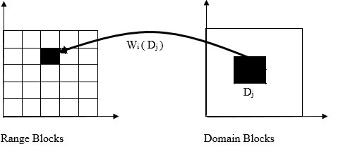
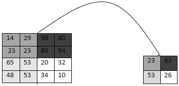
where # is the number of elements in the set, (k, l) the coordinates with gray level i, (m, n) the coordinates with gray level j. The following Fig. 1 illustrates the above definitions of a co-occurrence matrix (d=1, ? = 0 0 ).
Even though Haralick extracted 24 parameters from co-occurrence matrix, the present paper used only energy, contrast, local homogeneity, and correlation as given in Equations ( 2) to (5).
Energy = ? ?ln??? ???? ? 2 ???1 ??,?? =0 (2)Energy measures the number of repeated pairs and also measures uniformity of the normalized matrix.
Contrast = ? ??? ???? (i ? j) 2 ???1 ??,?? =0(3)The contrast feature is a difference moment of the P matrix and is a standard measurement of the amount of local variations present in an image. The higher the value of contrast are, the sharper the structural variations in the image.
Local Homogenity = ? ? ?? ???? 1+(i?j) 2 ? ???1 ??,?? =0(4)It measures the closeness of the distribution of elements in the GLCM to the GLCM diagonal. The converse of homogeneity results in the statement of contrast.
Correlation = ? ??? ???? (i??)(j??) (?) 2 ? ???1 ??,?? =0(5)Where P ij is the pixel value in position (i, j) of the texture image, N is the number of gray levels in the image,
? is ? = ? i?? ???? N?1 i,j=0mean of the texture image and (?) 2 is (?
) 2 = ? ?? ???? (i ? ?) 2 ???1 ??,?? =0variance of the texture image. Correlation is the measure of similarity between two images in comparison. The measures mean (m), which represents the average intensity.
4. III. textons
Textons [30,31] are considered as texture primitives, which are located with certain placement rules. A close relationship can be obtained with image features such as shape, pattern, local distribution orientation, spatial distribution, etc. using textons. The textons are defined as a set of blobs or emergent patterns sharing a common property all over the image. The different textons may form various image features.
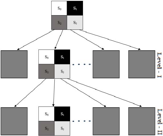
To have a precise and accurate texture classification, the present study strongly believes that one need to consider all different textons. That is the reason the present study considered all. There are several issues related with i) texton size ii) tonal difference between the size of neighbouring pixels iii) texton categories iv) expansion of textons in one orientation v) elongated elements of textons. By this sometimes a fine or coarse or an obvious shape may results or a pre-attentive discrimination is reduced or texton gradients at the texture boundaries may be increased. The present paper utilized the following five texton shades of 2×2 grid shown in Fig. 2. In Fig. 2 Blob shape (Index =5): TU 15 with all 1's represents a blob shape as shown in Fig. 8. The advantage of SDI is they don't depend on relative order of texture unit weights and can be given in any of the four forms as shown in Fig. 9 where the relative TU will change, but shape remains the same. 4 along with a bar graph shown in Fig. 19. The Table 5 compares discrimination rates of our earlier methods Texton based Cross Shape Descriptor Index (TCSDI) Texton based Diagonal Shape Descriptor Index (TDSDI) [ 2,4 ] with the current method TTSCM approach of this paper. The corresponding bar graph representation is shown in Fig. 20.
5. The
proposed TTSCM obtained high discrimination rate over our earlier TCSDI and TDSDI methods. This is because the TTSCM represent the SDI of the entire image instead of two separate or partial images of TCSDI and TDSDI.


| Texture numbe r | Contras t | Correlat ion | Energy | Homog eneity |
| E_1 | 9.159 | 0.3525 | 0.032 | 0.4971 |
| E_2 | 9.809 | 0.3369 | 0.0354 | 0.5044 |
| E_3 | 9.129 | 0.3472 | 0.0375 | 0.5137 |
| E_4 | 9.268 | 0.3631 | 0.0375 | 0.5165 |
| E_5 | 8.801 | 0.3546 | 0.0387 | 0.5187 |
| E_6 | 9.187 | 0.3343 | 0.0371 | 0.5156 |
| E_7 | 7.254 | 0.2813 | 0.0474 | 0.5335 |
| E_8 | 6.479 | 0.2645 | 0.0509 | 0.5414 |
| E_9 | 12.69 | 0.4056 | 0.0324 | 0.5063 |
| E_10 | 6.252 | 0.2921 | 0.0495 | 0.5478 |
| Texture numbe r | Contras t | Correlati on | Energy | Homog eneity |
| W_1 | 18.74 | 0.4686 | 0.0402 | 0.5306 |
| W_2 | 16.83 | 0.3171 | 0.0327 | 0.4965 |
| W_3 | 15.08 | 0.328 | 0.0352 | 0.5022 |
| W_4 | 17.71 | 0.3615 | 0.0345 | 0.4859 |
| W_5 | 18.45 | 0.4389 | 0.0301 | 0.5002 |
| W_6 | 12.03 | 0.314 | 0.0359 | 0.5031 |
| W_7 | 16.48 | 0.4387 | 0.0317 | 0.5013 |
| W_8 | 15.26 | 0.5095 | 0.0408 | 0.5462 |
| W_9 | 16.43 | 0.3591 | 0.0316 | 0.5024 |
| W_10 | 19.39 | 0.3411 | 0.027 | 0.4851 |
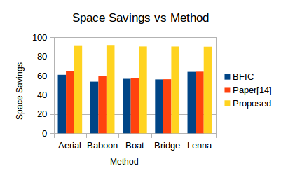
| Methods | Average discrimination rates (%) |
| TCSDI | 84.33 |
| TDSDI | 88.66 |
| TTSCM | 93 |
| Texture Database | Discrimination rate (%) TTSCM method |
| Elephant | 93 |
| Car | 100 |
| Water | 86 |
| Average Discrimination rate | 93 |
| original image one representing the cross and other | |
| representing the diagonal features. |