1.

Borehole ballooning sometimes referred as breathing is an expression used to describe the small volumetric change of the active drilling fluid system, which might occur during drilling operations. The phenomenon of borehole ballooning is caused mainly by following mechanisms [[1], [2]]:

? Thermal expansion and contraction of the drilling fluid. ? Compressibility of the drilling fluid.

? Elastic deformation of the borehole and the cased hole.

? The opening and closing of induced fractures at the near wellbore region. ? The opening and closing of natural fractures intersected during drilling. By estimating the change in volume of the wellbore caused by one of above mentioned processes, we can avoid confusion with conventional losses or formation kick, consequently nonproductive time (NPT) is reduced.

2. H

sensitivity study using syntactic data in order to investigate the effects of different parameters on volumetric deformation of the open borehole, the outcome of the study clearly shows that the volume variation is insignificant and controlled by the drilling fluid weight and temperature [5].

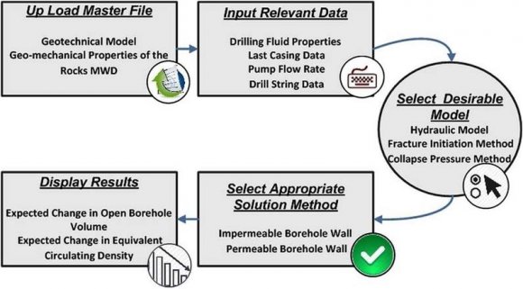
This paper presents standalone software (built on Matlab) to predict and quantify the volumetric change of the active drilling fluid system due to elastic deformation of the open borehole wall, which will assist the drilling engineers to a certain extent to avoid mixing ballooning with other formation flow incidents such as kick or loss. The developed software was designed to fully utilize the existing Geotechnical Mode land rock geo-mechanical properties for any depth interval in order to execute the main objectives of the tool. The the elastic deformation of an open borehole wall, the equations have been validated numerically; this paper presents the recent work of Elmgerbi et al, which is exemplified in standalone software. Generally, the software has multiple features and it is capable to estimate the volumetric change of an open borehole section for different conditions and multi layers by using the Geotechnical Model data such as in situ principal stresses gradients and pore pressure gradient in addition to geo-mechanical properties of the rock like, Poisson's ratio, Young's modulus. The graphical user interface of the software (GUI) has been designed in a manner that allows the user to execute the entire process easily within a short time. The working sequence of the tool consists of five phases, data uploading, data inputting, model selection, final execution and result displaying. Since the graphical analysis is always preferable hence the software generates multiple figures, these figures collectively are comprehensive and readable that leads to valuable analysis. Figure 1depicts the process roadmap of the developed software.

3. III. Processing Steps a) Data Uploading

Three different data sources are combined in one file (Master file), Geotechnical Model, geomechanical properties of the rocks and subsurface data. Therefore it is assumed that the Geotechnical Model and rock properties of the interested field have been [6].Table 1 shows the essential data categories and sources. already obtained. Building a Geotechnical model can be derived by gathering and analyzing, wire line logs data, down hole measurements data, and drilling experiences, whereas the rock properties can be determined by combing logs data with laboratory tests Recently Elmgerbi et al [5]introduced new analytical equations which are used primarily to predict variation [3]. Helstrup et al (2001) stated that change in borehole volume due to elastic deformation can be significant and it is mainly driven by wellbore radius, well pressure and Poisson's ratio. Their results show that the change in volume can be as high as 1 bbl for 100 meter depth interval [4].On 2016 Asad et al performed The Master file, which is recognized by the tool, is a structured text file containing fifteen channels and header information. The header information is located at the beginning of the file and followed by data arrays.

4. II. Background

5. b) Data Entry

In the data entry phase the users is allowed to add more information in order to allow effective and successful processing and ensure the integrity of the results. The required data here is particularly related to well, which is under the study.

6. IV. Mathematical Models and Methods

The tool allows the user to choose the desirable hydraulic model and the appropriate failure criteria for both compressive and tensile conditions. Therefore several equations have been integrated with tool. In the next section the utilized equations will be presented.

7. a) Hydraulic Models

The three known hydraulic models, Bingham, Power law and Herschel Bulkley have been integrated with the software in order to make it independent. The main role of the hydraulic model here is to predict the annular pressure loss for the open and cased sections. The table below shows the pressure loss equations used by the software. Full mathematical derivations of the entire equations can be found in reference [8]. Year 2016 ( )

= PV * ? 1000 * (D 2 ? D 1 ) 2 + Y p 200 * (D 2 ? D 1 )

(1)

Turbulent P ?? = ? 0.75 * ? 1.75 * PV 0.25 1396 * (D 2 ? D 1 ) 1.25(2)

Power law

Laminar P l = ? 144 * ? D 2 ? D 1 * 2 * n + 1 3 * n ? n * 0.00208 * k 300 * (D 2 ? D 1 )(3)Turbulent P l = f * ? * ? 2 21 . 1 * (D 2 ? D 1 )(4)

8. Herschel Bulkley

Laminar

P l = ? 0.09984 * k 14400 * (D 2 ?D 1 ) ? * ? Y p 0.00208 * k + ?? 192 * (2 * n+1) n * C a * (D 2 ?D 1 ) ? * ? 0.1016 * Q (D 2 2 ?D 1 2 ) ?? n ?(5)

Turbulent

P ?? = 7.48 * f * (0.002217 * Q) 2 * ? 0.005712 * (D 2 ? D 1 ) * (D 2 2 ? D 1 2 ) 2 (6)

9. b) Fracture Initiation Pressure and Collapse Pressure Methods

In case the Geotechnical Model does not include fracture initiation pressure and collapse pressure, the software offers several methods, which can be used to predict upper and lower bounds of the safe mud pressure window. [13], [14] Mohr Coulomb

Case#1

p wc = ?3? H ? ? h + ? t ?t ? * ?1 ? SIN(?)? 2 ? S o * COS(?) + ?? * P p ? * SIN(?)(12)

Case#2 p wc = 1

?1 + SIN(?)? * ?(? v + ? t ?t + 2 * ?(? H ? ? h )) * ?1 ? SIN(?)? ? 2 * S o * COS(?) + ?? * P p ? * SIN(?)?(13)

Modified Lade

I 3 = I 1 3 (27 + ?)(14)

10. H

The detailed steps for deriving the equations can be found in Appendix

11. c) Stress Transformation Equations

In case the borehole is horizontal or inclined, the stress transformation equations are triggered in order to transform the stresses to a new Cartesian coordinate system, where two stresses are perpendicular to the borehole whereas the third stress is parallel to the axes of the borehole [15].

? H °= ?? H * ?COS(?)? 2 + ? h * ?SIN(?)? 2 ? * ?COS(?)? 2 + ? v * ?SIN(?)? 2 (15)? h °= ?? H * ?SIN(?)? 2 + ? h * ?COS(?)? 2 ? (16)? v °= ?? H * ?COS(?)? 2 + ? h * ?SIN(?)? 2 ? * ?SIN(?)? 2 + ? v * ?COS(?)? 2 (17)? xy °= 1 2 (? H ? ? h ) * ?SIN(2?)? * ?COS(?)? (18) ? xz °= 1 2 ?? H * ?COS(?)? 2 + ? h * ?SIN(?)? 2 ? ? v ? * ?SIN(2?)? (19)

12. d) True Vertical Depth Determination Method

There are several known methods of computing true vertical depth, one of these methods is the minimum curvature, it is theoretically the most accurate and most commonly used, hence it was integrated with software [16]. e) Solution Methods Two solution methods are available, one is for impermeable borehole wall whereas the second for permeable. Practically, the impermeable proposed solution is valid once the rock formation is exposed to [Initial condition], whereas the permeable solution is effective only when a stable mud cake is built [Steady stat condition].Only the final formula of the two methods will be mentioned here. Therefore for more details refer to reference [5]. the drilling fluid and last as long as no filtration occurs

u = r * 1 E ?P w * (1 + ?) ? (? * P w ) * (2? ? 1) ? (1 ? ?) * ?? t ?t + 2? ?P w ? ?? * P p ??? ? (? 2 ? 1) * ?2(? H ? ? h ) COS(2?) + 4 * ? xy * SIN(2?)? ? ? H ? ? h + ? * ? v ? (23) Impermeable u = r * (1 + ?) E ?P w ? (2? ? 1) (1 + ?) * ?? * P p ? ? (1 ? ?) (1 + ?) * ? t ?t ? 1 (1 + ?) * (? H + ? h ? ? * ? v ) ? 2 * (? ? 1) * ?(? H ? ? h ) COS(2?) + 2 * ? xy * SIN(2?)?? (24)

13. H

V. Deliverables of the Software Several figures are generated, which would assist to improve individual analysis quality and provide a simple visual way of analyzing. The following points show the main figures that displayed by the developed software:

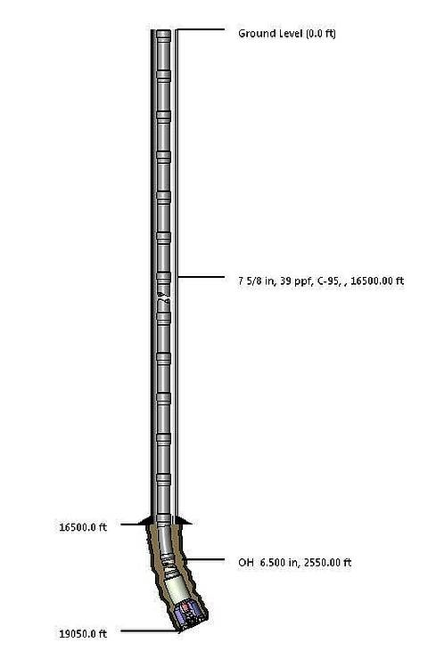
? Well profile.

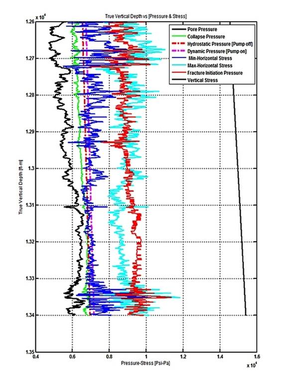
? Safe mud pressure window.

? Volumetric change of the open borehole section.

? Change in the Equivalent Circulating Density (ECD).

? Open borehole section condition.

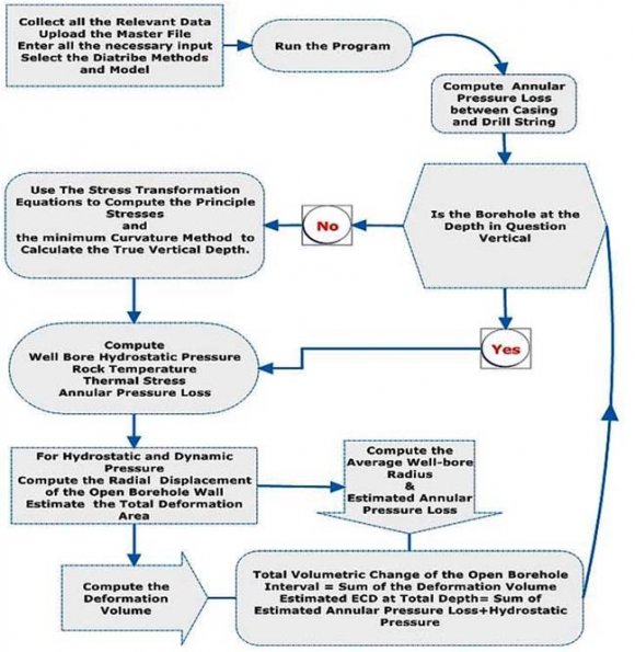
14. VI. Internal Workflow Description

Sequential steps are performed at the back ground of the software in order to achieve the main objectives of the software. Figure 2below depicts these steps. As it is illustrated in Figure 2, the process starts by computing the annular pressure loss between the casing and drill string, here the given casing depth and drill string geometry are used. Then the software starts fetching the data point from the master file, one by one, each time several steps are performed, the steps are repeated for each single data point till the last data

15. VII. Case Study

Necessary analysis for the presented case study performed using historical data belonging to two wells.

The main objectives of the study were to measure the effects of different controllable and uncontrollable parameters on the volumetric changes of the open borehole section and to evaluate any expected changes which would occur to ECD saccordingly. The initial well condition for the example mentioned can be seen in Table 8.

16. E a r l y

V i e w ? In first scenario, the initial well condition was applied (Table 8).

? In the second scenario, the effect of the mud weight was investigated.

? In the third scenario, the influence of drilling fluid temperature was studied.

In each scenario the pump flow rate was gradually increased from the initial rate to maximum allowable rate. As it is clearly indicated in Figure 4, this well can be characterized as the one with narrower safe mud pressure window consequently the maximum permissible pump flow rate was limited to1000 gpm. Figure 5depicts the results of the studied scenarios. In general, the volumetric change of the open borehole section and change in ECD increase with increasing the pump flow rate. However the changes are not significant and they can be ignored. Although in second scenario the mud weight was higher, it did not make remarkable changes, the reason for that mainly related to the contraction and expansion of the open borehole, in all scenarios, the borehole was always in contraction status even with higher flow rate [Figure 6]. The results show another important observation that the change in ECD in second scenario is always less comparing to the other scenarios, again the main reason of that is the borehole condition. Increasing mud weight would intend to change the borehole from contraction condition to expansion condition, hence the average radius of the deformation borehole increases and the cumulative annular pressure loss at the bottom of the borehole decreases accordingly. Comparing the third scenario with first scenario, slight increase in the volumetric change of the open borehole section can be noted, it is caused mainly by the thermal stress. The existence of the thermal stress will cause the drillinduced stresses to increase, consequently the open borehole shrinks and the annular pressure loss increases. Therefore, higher dynamic wellbore pressure is expected, it cause the open borehole section to expand, due to this expansion, the difference in deformation volume between the pump on and off is higher.

17. Conclusion

The main conclusion of the presented work can be summarized in the following points:

? For the purpose of accurately quantifying the volumetric change of an open borehole section and its impact on the hydraulic system, Standalone software has been developed, it has multiple features and it is able to estimate the volumetric change of an open borehole section and to predict any possible change might occur to the ECD for any given well by utilizing the Geotechnical Model data, geo-mechanical properties of the rocks and subsurface data.

? Detailed description for all the equations and models of the developed software have been provided. ? Since the graphical analysis is always preferable hence the developed software generates multiple charts, these charts collectively are comprehensive and readable that leads to valuable analysis.

? The findings of two case studies can be concluded as following:

o The elastic deformation of an open borehole section wall certainly occurs and its severity

? The slight increase in volumetric change and the change in ECD in the third scenario are due to the thermal stress effect.

negative, in other words, the predicted ECD at the bottom of the hole is less than the theoretical ECD.

in situ principal stresses and the drilling fluid weight.

I. Introduction ertainly, three processes can cause volumetric changes to the active drilling system, these process are: ? Kick: A flow of formation fluids into the wellbore during drilling operations. ? Loss: The leakage of the liquid phase of a drilling fluid, slurry or treatment fluid containing solid particles into the formation matrix. ? Borehole breathing (Ballooning). — Figure 1.

Figure 1: Process Roadmap of the Developed Software. — Figure 2. Figure 1 :

DL = COS ?1 * [SIN(? 1 ) * SIN(? 2 ) * COS(? 2 ? ? 1 ) + COS(? 1 ) * COS(? 2 )](20) — Figure 3.

Figure 2 : Internal Workflow of the Developed Software — Figure 4. Figure 2 :

Figure 3 : Wellbore Schematic — Figure 5. Figure 3 :

Figure 4 : Safe Mud Pressure Window — Figure 6. Figure 4 :

Figure 5 : Expected Change in Open Borehole Volume and ECD for Different Pump Flow Rate [Well A] [In the second scenario the mud weight was increased to 10.5 ppg instead of 10 ppg, while in third scenario, the drilling fluid temperature is assumed to be 127?C for the entire open hole section and 0. 925 [?C/100ft] used as thermal gradient]The results show another important observation that the change in ECD in second scenario is always less comparing to the other scenarios, again the main reason of that is the borehole condition. Increasing mud weight would intend to change the borehole from contraction condition to expansion condition, hence the average radius of the deformation borehole increases and the cumulative annular pressure loss at the bottom — Figure 7. H[Figure 5 :

Figure 6 : Cumulative Deformation Volume of the Open borehole section for Different Pump Flow Rate [Well A] — Figure 8. Figure 6 :

Figure 7: Expected Change in Open Borehole Volume and ECD for Different Pump Flow Rate [Well B] [In the second scenario the mud weight was increased to 13.5 ppg instead of 11.5 ppg, while in third scenario, the drilling fluid temperature is assumed to be 177?C for the entire open hole section and 0. 925 [?C/100ft] used as thermal gradient] — Figure 9. Figure 7 :

Figure 8: Cumulative Deformation Volume of the Open Borehole Section for Different Pump Flow Rate [Well B] [It is obvious that the open borehole is under contraction status in first and third scenario, in contrast it is under expansion status in the second scenario.] VIII. — Figure 10. Figure 8 :

Figure 11. Table 1 :

Category	Parameter	Sources
Geotechnical Model	Vertical Principal Stress. Intermediate Principal Stress. Least Principal Stress. Pore Pressure.	Density and Soniclogs, Cuttings. Image and caliper logs, failure analysis. Leak-off tests, extended leak-off tests, Sonic logs. Sonic, resistivity and density logs, seismic data.
	Young's Modulus.	Bulk density log, laboratory core tests, cavings.
	Poisson Ratio.	Bulk density log, laboratory core tests, cavings.
Rock Properties	Biot Constant. Thermal Expansion Coefficient. Laboratory core tests. Laboratory core tests. Cohesive Strength. Laboratory core tests.
	Friction Angle.	Bulk density log, laboratory core tests.
	Tensile Strength.	Laboratory core tests.
	Measured Depth.	Rig Data.
Well Data	Hole Inclination. Hole Azimuth.	Measuring while drilling. Measuring while drilling.
	Expected Mud Temperature.	Logs.

Figure 12. Table 2 :

Model	Flow Regime	Pressure Loss
	Laminar P ??
Bingham

Figure 13. Table 3 :

Method				Fracture Initiation Pressure
Hubbert & Willis	?? ð??"ð??" =	?1 ? ??????( ?)? ? 1 + ??????(?)?		??? ?? ? ?? * P p ?? + ?? * P p ?	(7)
Eaton	?? ð??"ð??" =	?? (1 ? ??)	??? ?? ? ?? * P p ?? + ?? * P p ?		(8)
Minimum Stress	?? ð??"ð??" = ? h				(9)
Bellotti &Giacca ??? Hoop Stress Method ?? ð??"ð??" = 2 * ?? (1 ? ??) P f = 3??

Note: ?? ? ?? * P p ?? + ?? * P p ? (10) ? ? ?? ?? ? ?? * P p ? + ? t ?t + T(11)

Figure 14. Table 4 :

Figure 15. Table 5 :

Stress Transformation Equations

Figure 16. Table 6 :

Minimum Curvature Method

Figure 17. Table 7 :

Radial Elastic Displacement

Permeable

Figure 18. Table 8 :

Well A

Well B

Figure 19.

		depends on geotechnical properties of Nomenclature
	P l	encountered formation, magnitude of the in situ Pressure Loss [Psi/ft, Pa/m]
	?	principle stresses, induced stresses, well Density [ppg]
	geometry, well profile and the operational PV Plastic viscosity [cP]
	?	margin between dynamic and the hydrostatic Mean velocity [Ft/second]
	pressure. Y p		Yield point [Ib/100ft²]
	o The volumetric change of the open borehole D 1 Drill string outer diameter [in, m ]
	section and change in ECD increase with D 2 Casing inner diameter, open hole diameter [in, m]
	n	increasing the pump flow rate. Behavior Index [Dimensionless]
	k o The static condition [pump off] of an open Consistency Index [EqcP] f Friction Factor [Dimensionless] borehole section in terms of contraction and expansion is mainly driven by the status of the Herschel Bulkley variable [Dimensionless] C a Q Flow rate [gpm, m 3 /second]
	?? ð??"ð??"		Fracture initiation pressure [Psi,Pa]
	?		Rock frication angle [?]
	?? ??		Vertical principle stress [Psi,Pa]
	?		Biot's elastic constant [Dimensionless]
	P p		Formation pore pressure [Psi,Pa]
	??	Poisson ratio [Dimensionless]
	? h		Minimum horizontal principle stress [Psi,Pa]
	?? ?? ? t ?t		Maximum horizontal principle stress [Psi,Pa] Thermal stress [Psi,Pa]
	T		Rock tensile strength [Psi,Pa]
H	p ???? ? The second possible situation occurs if the Collapse pressure [Psi,Pa] S o Rock cohesive strength [Psi,Pa] open borehole condition changes from contraction to expansion, in this casethe First stress invariant [Psi,Pa] I 1 I 3 Third stress invariant [Psi 3 ,Pa 3 ] predicted ECD will be less than the ? Material parameter related to friction [Dimensionless] theoretical ECD and consequently the change in ECD will be negative. ?? 11 Major effective principal stress [Psi,Pa] ?? 22 Intermediate effective principal stress [Psi,Pa]
	?? 33		Minor effective principal stress [Psi,Pa]
	? rr		Effective radial stress
	? ??		Effective tangential stress
	? zz		Effective stress along the borehole axis
	??	Angle around the borehole measured anticlockwise from the azimuth of?? ??
	? ?z		Shear stresse in [??,z] plane [Psi,Pa]
	? xz		Shear stresses in [x,z] plane [Psi,Pa]
	? xy		Shear stresses in [x,y] plane [Psi,Pa]
	? yz		Shear stresses in [y,z] plane [Psi,Pa]
	S 1		Material parameter [Psi,Pa]
	u	Radial elastic displacement for the borehole [in, m ]
	r	Wellbore radius [in, m ]
	E		Young's modulus [Psi,Pa]
	?	Poroelastic stress coefficient [Dimensionless]
	P w		Borehole Pressure [Psi,Pa]

Appendix A

Appendix A.1 Appendix

Mohr Coulomb General failure Equation is; ?? 11 ? ?? 33 = 2 * ?? ?? * ??????(?) + (?? 11 + ?? 33 ) * ??????(?)(A1) Well bore collapse is expected to occur at the azimuth of ? h , in other word at ??=90? , hence the induced stresses can be calculated using the following equations; ? rr = P wc ? ?? * P p (A2) Insert EqA2 and A3 into Eq A1, after few mathematical steps and arrangements we end up with the following Equation for collapse pressure:

In case two the following condition is assumed ?? ???? ? ?? ???? ? ?? ???? Therefore in Eq A1 ?? 11 = ?? ???? and?? 33 = ?? ???? Now by inserting A2 and A4 into Eq A1 collapse pressure for the second case can be derived:

Because the collapse occurs at ??=90?, Eq A9 and A10 for cylindrical coordinate will have the following forum:

I 1 = (? rr + S 1 ) + (? ?? + S 1 ) + (? zz + S 1 (A13) I 3 = (? rr + S 1 ) * (? ?? + S 1 ) * (? zz + S 1 ) ? (? rr + S 1 )? ?z (A14) By substituting ? rr , ? ?? , ? zz and ? ?z in Eq A13 and A14 with Eq A2, A3, A4 and A5 respectively Now back to Eq A8 rearrange it

Finally replace?? 1 , ?? 3 , ?? 1 and ?? with Eq A15,A16,A11 and A12 respectively in Eq A8, the right side of Eq A8 is independent of P wc , while the left side is a quadratic expression in P wc . Therefor by solving Eq A8 the collapse pressure P wc can be obtained. Since two solutions are expected, the collapse pressure equals the lesser one.

Appendix A.2 This page is intentionally left blank

Appendix B

Fracture Gradient Prediction and Its Application in Oilfield Operations. A Ben , E . 10.2118/%2087223-PA. http://dx.doi.org/10.2118/21 Journal of Petroleum Technology October 1969. 21 p. 63. (Issue 10, 8 pages)
General Analytical Solution for Estimating the Elastic Deformation of an Open Borehole Wall. A Elmgerbi , G Thonhauser , M Prohaska . http://www.ijser.org/onlineResearchPaperViewer.aspx International Journal of Scientific & Engineering Research January 2016. 7. (Issue 1, 13 pages)
A Practical Method for Evaluating Effects of Fracture Charging and/or Ballooning When Drilling High Pressure. A Helstrup , M K Rahman , M M Hossain , S Rahman . 10.2118/67780-MS. http://dx.doi.org/10.2118/67780-MS High Temperature (HPHT) Wells. Presented at SPE/IADC Drilling Conference, (Netherlands, Amsterdam
) 2001. 27 February-1 March 2001. (SPE-67780-MS)
Watching Rocks Change-Mechanical Earth Modeling. Oilfield Review, Akbar Ali , A Brown , T Delgado , R . 10.2118/%2021%2063-PA. https://www.slb.com/~/media/Files/resources/oilfield.../p22_39.pdf 2013.
Mechanics of Borehole Ballooning in Naturally-Fractured Formations. A Lavrov , J Tronvoll . 10.2118/93747-MS. http://dx.doi.org/10.2118/93747-MS Presented at the SPE Middle East Oil & Gas Show and Conference, (Bahrain
) 2005. March 2005. p. . (SPE-93747-MS)
Mud Hydraulic Fundamentals. B Guo , G Liu . 10.2118/%2021%2063-PA. Applied Drilling Circulation System, 2011. Gulf Professional Publishing is an imprint of Elsevier. 2 p. . (first edition)
A Compilation of the Geo-Mechanical Properties of Rocks in Southern Ontario and the Neighbouring Regions. H El Al-Maamori , M Naggar , S Micic . 10.4236/ojg.2014.45017. dx.doi.org/10.4236/ojg.2014.45017 Open Journal of Geology April 2014. 4.
Temperature Model Provides Information for Well Control. K Eirik , S Aadnøy . http://www.ogj.com/articles/print/volume-96/issue-37/in-this-issue/drilling/temperature- Oil & Gas Journal September1998.
Mechanics of Hydraulic Fracturing. M K Hubbert , D G Willis . https://www.depts.ttu.edu/.../Hubbert%20and%20Willis,%201972%20me AIME Petroleum Transactions 1957. 210 p. .
Pressure evaluation improves drilling performance. P Bellotti , D Giacca . Oil and Gas Journal Sept. 11, 1978.
Wellbore-Stability Predictions by Use of a Modified Lade Criterion. R Ewy . 10.2118/84246-MS. http://dx.doi.org/10.2118/56862-PA Journal of Petroleum Technology June 1999. 14. (Issue 2, 7 pages)
Evaluation of ballooning in deep wells. S Aadnøy , S Brent . Modern Well Design, (London, Uk
) 2010. Taylor & Francis Group. 294. (second edition, Appendix B)
Stresses Around A Wellbore. S Aadnøy , R Looyeh . Petroleum Rock Mechanics Drilling Operations And Well Design, 2011. Elsevier. (first edition, Chapter10, 157: Gulf Professional Publishing is an imprint of)
A Compendium of Directional Calculations Based on the Minimum Curvature Method. Sawaryn , J Thorogood . 10.2118/84246-MS. http://dx.doi.org/10.2118/84246-MS Presented at the SPE Annual Technical Conference and Exhibition, (Denver, Colorado, U.S.A.
) 2003. 5 -8 October 2003. (SPE-84246)
Bounds on In-Situ Stress Magnitudes Improve Wellbore Stability Analyses. S Bernt , U Aadnøy . 10.2118/87223-PA. http://dx.doi.org/10.2118/87223-PA Journal of Petroleum Technology June 2005. 10. (Issue 2, 6 pages)
Wellbore/borehole stability. S Peng , J Zhang . 10.2118/56862-PA. Engineering Geology for underground Rocks, (Berlin, Germany
) 2007. Springer Science and Business Media. (first edition, Chapter7, 177)

Application of Computer Programming to Estimate Volumetric Change of an Active Drilling Fluid System Cause by Elastic Deformation of an Open Borehole Section Wall

Table of contents

1.