1. Introduction
mage segmentation is a fundamental task in many applications. Among various techniques, the active contour model is widely used. A contour is evolved by minimizing certain energies to match the object boundary while preserving the smoothness of the contour [2]. The active contour is usually represented by landmarks [18] or level sets [20,8]. A variety of image features have been used to guide the active contour, typically including image gradient [7,31], region statistics [34,8], color and texture [14].
In real purposes, the presentation of the active contour model is prone to be dishonored by missing or misleading features. For example, segmentation of the left ventricle in ultrasound images is still an unresolved problem due to the characteristic artifacts in ultrasound such as attenuation, speckle and signal dropout [23]. To improve the robustness of active contours, the shape prior is often used. The prior knowledge of the shape to be segmented is modeled based on a set of manuallyannotated shapes to guide the segmentation. Previous deformable template models [32,27,17,21] can be regarded as the early efforts towards knowledge-based segmentation. In more recent works, the shape prior was applied by regularizing the distance from the active contour to the template in a level-set framework [10,24,9]. Another category of methods popularly used for shape prior modeling is the active shape model or point distribution model [11]. Briefly speaking, each shape is denoted by a vector and regarded as a point in the shape space. Then, the principal component analysis is carried out to obtain the mean and several most significant modes of shape variations, which establish a low-dimensional space to describe the favorable shapes. During the segmentation of a new image, the candidate shape is constrained in the shape space [19,29]. Also, dynamic models can be integrated to model the temporal continuity when tracking an object in a sequence [12,35]. Other extensions of the active shape model include manifold learning [15] and sparse representation [3:5], to name a few.
While the shape prior has proven to be a powerful tool in segmentation, it has two limitations: 1. Previous methods for shape prior modeling require a large set of annotated data, which is not always accessible in practice. 4. We applied the proposed method to sequence of surveillance face images and demonstrated that the Diminutive sequence optimality regularization could significantly improve the robustness of the active contour model. The rest of this paper is organized as follows: Section 2 introduces the basic theory and the formulation of our method. Section 3 describes the algorithm to solve our model. Section 4 demonstrates the merits of our method by experiments. Finally, Section 5 concludes the paper with some discussions.
2. II.
3. Formulation a) Diminutive Sequence Optimality Measure
To apply a Diminutive sequence optimality constraint to active contours, a proper measure to estimate that any of images are akin to source is desired. Characteristically, the akin among two contours is measured by scheming the distances between the equivalent points on the contours, and the minuscule sequence optimality can be calculated by the sum of pair-wise distances among contours. The main drawback of this technique is that the contour distance is not invariant below akin transformation.
Here, we propose to use the matrix rank to measure the Diminutive sequence optimality of shapes. Suppose each shape is represented by a vector. Multiple shapes form a matrix. Intuitively, the rank of the matrix measures the correlation among the shapes. For example, the rank equals to 1 if the shapes are identical, and the rank may increase if some shapes change. Moreover, we can show that the shape matrix is still lowrank if the shape change is due to the akin transformation such as translation, scaling and rotation. For example, let vector
p n n C C C × ? ? has the following property 1 ([ ,..., ]) 6 n rank C C ? (1)Intrinsically, the rank of the shape matrix describes the degree of freedom of the shape change. The low-rank constraint will allow the global change of contours such as translation, scaling, rotation and principal deformation to fit the image data while truncating the local variation caused by image defects. segment the object in these images. To keep the contours similar to each other, we propose to segment the images by min 1 ( )
n X i i i f C = ? Subject to ( ) , rank X K ? (2) Where 1 [ ,..., ] n X C C = and K is a predefined constant. ( ) i if C Is the energy of an active contour model to evolve the contour in each frame, such as snake [18], geodesic active contour [7], and regionbased models [34,8]. For example, the region-based energy in [8] reads
1 2 2 2 1 2 ( ) ( ( ) ) ( ( ) ) ( ) i i i i i f C I X u dx I X u dx length C ? ? ? = ? + ? + * ? ?(3)Where 1
? and
4. 2
? represent the regions inside and outside the contour, and 1 u and 2 u denote the mean intensity of 1
? and 2 ? , respectively.Since rank is a discrete operator which is both difficult to optimize and too rigid as a regularization method, we propose to use the following relaxed form as the objective function:
min 1 ( ) n X i i i f C X ? * = + ? (4)Here, rank(X) in ( 2) is replaced by the central median X * , i.e. the sum of singular values of X.
Recently, the central median minimization has been widely used in low-rank modeling such as matrix completion [6 ] and robust principal component analysis [5 ]. As a tight convex surrogate to the rank operator [16 ], the central median has several good properties: Firstly, the convexity of the central median makes it possible to develop fast and convergent algorithms in optimization. Secondly, the central median is a continuous function, which is important for a good process of regularize in many applications. For instance, in our problem, the small perturbation in the shapes may result in a large increase of rank(X), while X * may rarely change.
5. Algorithm
In this section, we will discuss how to solve the optimization problem observed in (Eq4). If regularizing process not opted X * , (Eq4) can be locally minimized by changeover descent, which gives the curve evolution steps in typical active contour models. In our model, it is difficult to apply changeover descent directly due to the central median, which is coarse and its partial changeover is hard to compute.
( ) ( ) X F X R X ? + (5)Where ( ) F X a differentiable is function and ( ) R X corresponds to a convex penalty which can be coarse. Our problem is in this category with
1 ( ) ( ) n i i i F X f C = = ? and ( ) R X X * =.The basic step in Proximal Gradient is to make the following quadratic approximation to F(X) based on the previous estimate
' X per iteration. Add Eq 6 2 2 ( , ') ( ') ( '), ' ' ( ), 2 1 [ ' ( ')] ( ) 2 F F Q X X F X F X X X X X R X X X F X R X const µ µ ? µ ? µ = + ?? ? ? + ? + = ? ? ? + + ? ?(6)Where .,. ? ? means the inner product, . F denotes the Frobenius norm, and ? is a constant. It is shown in [22] that, if F(X) is differentiable with Lipschitz continuous gradient, the sequence generated by the following iteration will converge to a stationary point of the function in ( 5) with a convergence rate of
1 ( ) k ? . 1 2 min arg ( , ) 2 min 1 1 arg [ ( )] ( ) 2 2 k k k k F X Q X X X X F X R X µ ? µ µ + = = ? ? ? +(7)The next question is how to solve the update step in (Eq7). For our problem, the lemma proven in [4] has been taken to define the proposed hastened propinquity changeover algorithm.
6. Lemma 1 Given
, the solution to the problem
2 * min 1 2 F X Z X X ? ? +(8)is given by
* ( ) X D Z ? =, where
min( , )1( ) ( ) m n T i i i i D Z u v ? ? ? = = ? + ?(9)The intuition of our algorithm is that, per iteration, we first evolve the active contours according to the image-based forces and then impose the Diminutive sequence optimality regularization via singular value threshold. The overall algorithm is summarized here. Hastened propinquity changeover algorithm 2. 0 fork = ? Maximum number of iterations do 3.
1 1
7. ( )
8. Performance Analysis and Results Exploration
In this section, we evaluate the proposed method on both synthesized data and surveillance face image sequence. To demonstrate the advantages of the Diminutive sequence optimality constraint, we compare the results of the same active contour model before and after applying the proposed constraint. We select the region-based active contour in (3) as the basic model, which is less sensitive to initialization and has fewer parameters to tune compared with edge-based methods.
In our execution, we initialize the energetic contours as
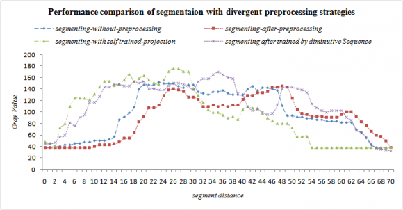
0 0,..., 0 [ ] X C C =, where 0 C is a coarse outline of the object placed manually in an image. Three parameters need to be selected in our algorithm. ? in (Eq3) controls the smoothness of each contour, ? in Recently, the Proximal Gradient (PG) method [1,22] is used to solve the following category of problems 1. The bottom row of figure 2 indicates the results obtained from different strategies. There are two comments worth mentioning. Firstly, the contour shapes are globally consistent with each other throughout the sequence, which is attributed to the Diminutive sequence optimality constraint. Hence, the contours are more resistant to local misleading features. Secondly, the constrained shape model is still flexible enough to adapt the deformation of the object shape. The problem of our method is that it cannot address the universal bias of the model. Therefore, the region-based active contours cannot attach closely to the true boundary. In practice, more appealing results can be obtained by including more energy terms such as edge-based energies, which is out of the scope of this paper. The results are summarized in Table 1. Regarding the mean of the metrics, a smaller MAD/HD or a larger Dice coefficient indicates a more accurate segmentation. Generally, the performance with the proposed constraint is better than that without the constraint. The improvement in the diminutive sequence trained distance is the most notable, which measures the largest error for each contour. This is due to the fact that part of the segmentation result is corrupted by the missing boundary while this error can be corrected by adding the shape constraint. Regarding the standard deviation of the metrics, a smaller standard deviation indicates the more stable performance. The standard deviation with the proposed constraint is distinctly lower than that without the constraint, which shows the significance of the proposed constraint to improve the robustness of the active contour model. In our experiments, we selected ? empirically and applied the same ? to all sequences. The curve in Figure 4 shows that the accuracy changes smoothly over ? and the performance is stable in a wide range. Another alternative way is to choose a constant K specifying the degree of freedom allowed for shape variation and then solve the model with a decreasing sequence of ? until ( ) rank X reaches K.
9. d) Convergence and Computational Time
Our algorithm is executed in java and tested on a desktop through a Intel i7 3.4GHz CPU and 3GB RAM. The experiments showed that the algorithm with the shape constraint converged faster than that without shape constraint. This can be explained by the fact that the added constraint will make the active contour model better regularized, which results in faster convergence and fewer iterations. The results indicating that the algorithm with the proposed constraint is even faster in computation compared to that without the constraint.
V.
10. Conclusion
In this paper, we proposed a simple and effective way to regularize the Diminutive sequence optimality of shapes in the active contour model based on low-rank modeling and rank minimization. We use the position similarities to represent the contour instead of level sets. The reason is that the low-rank property in (Eq1) will not hold if the level-set representation is used. For instance, if there are n contours represented by the zero-level sets of n signed distance functions (SDFs) and the contours are identical in shape but different in location, the matrix consisting of the vector SDFs has a rank of n, which is full-rank. Other divergent methods for image segmentation also have this issue. A limitation of using the shape akin constraint is the possibility of removing frame-specific details of the shapes. The trade-off between noise removal and signal preserving is a fundamental challenge in many problems. A possible solution in our problem is to refine the segmentation by running an active contour model that is more sensitive to local features with our results being both initialization and templates to constrain the curve evolution. In future the formation and projection of the missing contour structure can be done by determining through support vector machines, which trained by the optimal contour features of the diminutive sequence.


| Projecting Active Contours with Diminutive Sequence Optimality | |||||
| Segmenting-Without- | Segmenting-After- | Segmenting-with Self | Segmenting after Trained | ||
| Distance | Preprocessing | Preprocessing | Trained-Projection | by Diminutive Sequence | |
| 0 | 37.6667 | 37.6667 | 47.4921 | 44.8643 | |
| 1 | 37.6667 | 37.6667 | 45.0357 | 44.8643 | |
| 2 | 40.0941 | 37.6667 | 40.123 | 47.2636 | |
| 3 | 40.0941 | 37.6667 | 72.0556 | 56.8605 | |
| 4 | 42.5216 | 37.6667 | 79.4246 | 59.2597 | |
| 5 | 42.5216 | 37.6667 | 108.9008 | 80.8527 | |
| 6 7 | 44.949 44.949 | 37.6667 37.6667 | 123.6389 123.6389 | 76.0543 90.4496 | 013 |
| 8 9 10 | 47.3765 47.3765 49.8039 | 37.6667 37.6667 40.0659 | 123.6389 121.1825 131.0079 | 116.8411 116.8411 95.2481 | Year 2 |
| 11 | 49.8039 | 42.4651 | 143.2897 | 126.438 | |
| 12 | 49.8039 | 42.4651 | 153.1151 | 143.2326 | |
| 13 | 52.2314 | 42.4651 | 153.1151 | 143.2326 | |
| 14 | 57.0863 | 44.8643 | 145.746 | 148.031 | |
| 15 | 86.2157 | 47.2636 | 148.2024 | 148.031 | |
| 16 | 91.0706 | 54.4612 | 155.5714 | 145.6318 | |
| 17 | 98.3529 | 54.4612 | 165.3968 | 145.6318 | |
| 18 | 108.0627 | 64.0581 | 153.1151 | 152.8295 | |
| 19 | 139.6196 | 83.2519 | 158.0278 | 150.4302 | |
| 20 | 146.902 | 92.8488 | 162.9405 | 152.8295 | |
| 21 | 146.902 | 107.2442 | 155.5714 | 140.8333 | |
| 22 | 146.902 | 107.2442 | 150.6587 | 140.8333 | |
| 23 | 151.7569 | 112.0426 | 148.2024 | 138.4341 | |
| 24 | 149.3294 | 128.8372 | 155.5714 | 138.4341 | |
| 25 | 149.3294 | 138.4341 | 170.3095 | 145.6318 | |
| 26 27 | 149.3294 144.4745 | 140.8333 138.4341 | 175.2222 175.2222 | 150.4302 150.4302 | ( D D D D D D D D ) F |
| 28 | 142.0471 | 136.0349 | 170.3095 | 148.031 | |
| 29 | 146.902 | 126.438 | 170.3095 | 145.6318 | |
| 30 | 146.902 | 126.438 | 140.8333 | 138.4341 | |
| 31 | 134.7647 | 121.6395 | 128.5516 | 152.8295 | |
| 32 | 132.3372 | 109.6434 | 116.2698 | 157.6279 | |
| 33 | 129.9098 | 109.6434 | 103.9881 | 157.6279 | |
| 34 | 134.7647 | 112.0426 | 99.0754 | 164.8256 | |
| 35 | 134.7647 | 109.6434 | 99.0754 | 169.624 | |
| 36 | 137.1922 | 112.0426 | 94.1627 | 164.8256 | |
| 37 | 132.3372 | 109.6434 | 89.25 | 160.0271 | |
| 38 | 129.9098 | 112.0426 | 91.7064 | 157.6279 | |
| 39 | 129.9098 | 112.0426 | 86.7937 | 131.2364 | |
| 40 | 129.9098 | 121.6395 | 103.9881 | 128.8372 | |
| 41 | 139.6196 | 128.8372 | 108.9008 | 109.6434 | |
| 42 | 144.4745 | 128.8372 | 106.4444 | 102.4457 | |
| 43 | 137.1922 | 133.6357 | 106.4444 | 104.845 | |
| 44 | 142.0471 | 133.6357 | 96.619 | 100.0465 | |
| 45 | 142.0471 | 136.0349 | 89.25 | 95.2481 | |
| 46 | 139.6196 | 143.2326 | 84.3373 | 97.6473 | |
| 47 | 137.1922 | 143.2326 | 79.4246 | 112.0426 | |
| 48 | 110.4902 | 145.6318 | 79.4246 | 140.8333 | |
| 49 | 93.498 | 143.2326 | 79.4246 | 143.2326 | |
| 50 | 93.498 | 124.0388 | 72.0556 | 143.2326 | |
| 51 | 91.0706 | 104.845 | 57.3175 | 140.8333 | |
| 52 | 91.0706 | 97.6473 | 57.3175 | 138.4341 | |
| 53 | 88.6431 | 95.2481 | 57.3175 | 133.6357 | |
| 54 | 88.6431 | 92.8488 | 37.6667 | 114.4419 | |
| 55 | 86.2157 | 92.8488 | 37.6667 | 107.2442 | |
| © 2013 Global Journals Inc. (US) | |||||