1. Introduction
arallel computing is a technique of executing multiple tasks simultaneously on multiple processors. The main goal of parallel computing is to increase the speed of computation. Efficient task scheduling & mapping is one of the biggest issue in homogeneous parallel computing environment [1]. The objective of Scheduling is to manage the execution of tasks in such a way that certain optimality criterion is met. Most scheduling algorithms are based on listscheduling technique [4] [6][2] [11]. There are two phases in List-scheduling technique: task prioritizing phase, where the priority is computed and assigned to each node in DAG, and a processor selection phase, where each task in is assigned to a processor in order of the priority of nodes that minimizes a suitable cost function. List scheduling algorithms are classified as static list scheduling if the processor selection phase starts after completion of the task prioritizing phase and dynamic list scheduling algorithm if the two phases are interleaved. A parallel program can be represented by a node-and edge-weighted directed acyclic graph (DAG) [2] [3]. The Directed Acyclic Graph is a generic model of a parallel program consisting of a set of processes. The nodes represent the application process and the edges represent the data dependencies among these processes.
This paper surveys various scheduling algorithms that schedule an edge-weighted directed acyclic graph (DAG), which is also called a task graph, to a set of homogeneous processors. We examine four classes of algorithms: Bounded Number of Processors (BNP) scheduling algorithms, Unlimited Number of Clusters (UNC) scheduling algorithms, and Arbitrary Processor Network (APN) & Task Duplication Based (TDB) scheduling algorithms. Performance comparisons are made for the BNP algorithms. We provide qualitative analyses by measuring the performance of these four BNP scheduling algorithms under useful scheduling parameters: makespan, speed up, processor utilization, and scheduled length ratio.
The rest of this paper is organized as follows. In the next section, we describe the generic DAG model and discuss its variations & techniques. A classification of scheduling algorithms is presented in Section 3.The four BNP scheduling algorithms are discussed in Section 4.The performance results and comparisons are presented in Section 5, Section 6 concludes the paper. Section 7 suggest about future scope of research.
2. II.
3. Task scheduling problem & model used
This section presents the application model used for task scheduling. The number of processors could be limited or unlimited. The homogeneous computing environment model is used for the surveyed algorithms. We first introduce the directed acyclic graph (DAG) model of a parallel program. This is followed by a discussion about some basic techniques used in most scheduling algorithms & homogeneous computing environment.
4. a) The DAG Model
The Directed Acyclic Graph [2][3] is a generic model of a parallel program consisting of a set of processes among which there are dependencies. The DAG model that we use within this analysis is presented below in Fig. 1 A task without any parent is called an entry task and a task without any child is called an exit task. A node cannot start execution before it gathers all of the messages from its parent nodes. The communication cost between two tasks assigned to the same processor is assumed to be zero. If node ni is scheduled to some processor, then ST(ni ) and FT(ni)denote the start-time and finish-time of ni, respectively.After all the nodes have been scheduled, the schedule length is defined as maxi{FT(ni)}across all processors. The node-and edge-weights are usually obtained by estimation. Some variations in the generic DAG model are:-Accurate model [2][3]-In an accurate model, the weight of a node includes the computation time, the time to receive messages before the computation, and the time to send messages after the computation. The weight of an edge is a function of the distance between the source and the destination nodes. It also depends on network topology and contention which can be difficult to model. When two nodes are assigned to a single processor, the edge weight becomes zero. Approximate model 1 [2][3] -Here the edge weight is approximated by a constant. A completely connected network without contention fits this model. Approximate model 2 [2][3]-In this model, the message receiving time and sending time are ignored in addition to approximating the edge weight by a constant.
An accurate model is useless when the weights of nodes and edges are not accurate. As the node and edge weights are obtained by estimation, which is hardly accurate, the approximate models are used. The approximate models can be used for medium to large granularity, since the larger the process grain-size, the less the communication, and consequently the network is not heavily loaded.
Preemptive scheduling: The preemptive scheduling is prioritized. The highest priority process should always be the process that is currently utilized.
Non-Preemptive scheduling: When a process enters the state of running, the state of that process is not deleted from the scheduler until it finishes its service time.
The homogeneous computing environment model is a set P of p identical processors connected in a fully connected graph [4]. It is also assumed that:
Any processor can execute the task and communicate with other processors at the same time.
Once a processor has started task execution, it continues without interruption, and on completing the execution it sends immediately the output data to all children tasks in parallel.
5. b) Basic Techniques in DAG Scheduling
Most scheduling algorithms are based on list scheduling. The basic idea of list scheduling is to assign priorities to the nodes of DAG, then place the nodes in a list called ready list according to the priority levels and then lastly map the nodes onto the processors in the order of priority. A higher priority node will be examined first for scheduling before a node with a lower priority. In case any two or more nodes have the same priority, then the ties are needed to be break using some useful method. There are various ways to determine the priorities of nodes such as HLF (Highest level First), LP (Longest Path), LPT (Longest Processing Time) and CP (Critical Path).Frequently used attributes for assigning priority are [2][4] [5]:t-level: t-level(Top Level) of the node ni in DAG is the length of the longest path from entry node to ni (excluding ni) i.e. the sum of all the nodes computational costs and edges weights along the path.
b-level: The b-level (Bottom Level)of a node ni is the length of the longest path from node ni to an exit node . The b-level is computed recursively by traversing the DAG upward starting from the exit node.
Static level: Some scheduling algorithms do not consider the edge weights in computing the b-level known as static b-level. or static level.
ALAP time: The ALAP (As-Late-As-Possible) start time of a node is measure of how far the node's start time can be delayed without increasing the schedule length. It is also known as latest start time (LST).
CP (Critical Path):It is the length of the longest path from entry node to the exit node A DAG can have more than one CP. b-level of a node is bounded by the length of a critical path.
EST (Earliest Starting Time): Procedure for computing the t-levels can also be used to compute the EST of nodes. The other name for EST is ASAP (As-Soon-As-Possible) start-time.
A DAG -G = (V, E, w, c) -that represents the application to be scheduled
6. Bnp scheduling algorithms
In this section, we discuss four basic BNP scheduling algorithms: HLFET, ISH, MCP, and ETF. All these algorithms are for a limited number of homogeneous processors. The major characteristics of these algorithms are summarized in Table 1 [6]. In table, p denotes the number of processors given.
7. Performance Results and Comparison
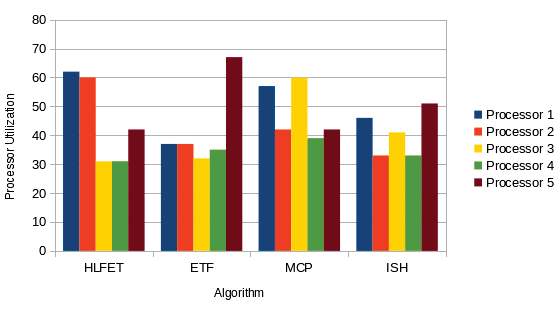
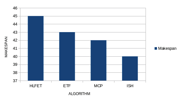
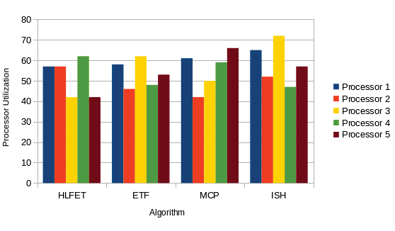
In this section, we present the performance results and comparisons of the 4 BNP scheduling algorithms discussed above. The comparisons are based upon the following four comparison metrics [2][4]: 1. Makespan: Makespan is defined as the completion time of the algorithm. It is calculated by measuring the finishing time of the exit task by the algorithm. 2. Speed Up: The Speed Up value is computed by dividing the sequential execution time by the parallel execution time.
1) Calculate the static b-level of each node.
2) Make a ready list in a descending order of static b-level. Initially, the ready list contains only the entry nodes. Ties are broken randomly. Repeat 3) Schedule the first node in the ready list to a processor that allows the earliest execution, using the non-insertion approach. 4) Update the ready list by inserting the nodes that are now ready. Until all nodes are scheduled.
8. 1) Calculate the static b-level of each node.
2) Make a ready list in a descending order of static b-level. Initially, the ready list contains only the entry nodes. Ties are broken randomly. Repeat 3) Schedule the first node in the ready list to the processor that allows the earliest execution, using the non-insertion algorithm. 4) If scheduling of this node causes an idle time slot, then find as many nodes as possible from the ready list that can be scheduled to the idle time slot but cannot be scheduled earlier on other processors. 5) Update the ready list by inserting the nodes that are now ready. Until all nodes are scheduled 1) Compute the ALAP time of each node.
2) For each node, create a list which consists of the ALAP times of the node itself and all its children in a descending order. 3) Sort these lists in an ascending lexicographical order. Create a node list according to this order. Repeat 4) Schedule the first node in the node list to a processor that allows the earliest execution, using the insertion approach. 5) Remove the node from the node list. Until the node list is empty.
9. 1) Compute the static b-level of each node.
2) Initially, the pool of ready nodes includes only the entry nodes. Repeat 3) Calculate the earliest start-time on each processor for each node in the ready pool. Pick the node-processor pair that gives the earliest time using the non-insertion approach. Ties are broken by selecting the node with a higher static b-level. Schedule the node to the corresponding processor. 4) Add the newly ready nodes to the ready node pool. Until all nodes are scheduled. So it can be concluded that for small number of tasks (35) MCP is the best algorithm but, with increasing number of tasks (50 & 65) ISH is one of the efficient algorithm, considering the data gathered using the scenarios and the performance calculated from them.
Future Scope: A lot of work can be done considering more case scenarios:
The number of tasks can be changed to create test case scenarios. Heterogeneous environment can be considered.

![{v i : i = 1,?., N } represents the set of tasks. E {e ij : data dependencies between node ni and node n j } w(n i ) represents the node n i 's computation cost (e ij )represents the communication cost between node n i and node n j . Level): Dynamic level of a node is calculated by subtracting the EST from the ST.III. A classification of dag scheduling algorithmsTheDAG scheduling algorithms are basically classified into the following four groups:a) B Bounded Number of Processors (BNP) scheduling [2][5][11]: BNP scheduling algorithms are non-task duplication based scheduling algorithms. These algorithms schedule the DAG to a bounded number of processors directly [2][5]. The processors are assumed to be fully-connected. No attention is paid to link contention or routing strategies used for communication. Most BNP scheduling algorithms are based on the list scheduling technique. Examples of BNP algorithms are: HLFET (Highest Level First with Estimated Times) algorithm, MCP (Modified Critical Path) algorithm, ISH (Insertion Scheduling Heuristic) algorithm, ETF (Earliest Time First) algorithm, DLS (Dynamic Level Scheduling) algorithm and LAST (Localized Allocation of Static Tasks). b) Unbounded Number of Clusters (UNC) scheduling [5][11]: UNC scheduling algorithms are non-task duplication based scheduling algorithms. The processors are assumed to be fully-connected and no attention is paid to link contention or routing strategies used for communication. The basic technique employed by the UNC algorithms is called Clustering. These algorithms schedule the DAG to an unbounded number of clusters. At the beginning of the scheduling process, each node is considered as a cluster. In the subsequent steps, two clusters are merged if the merging reduces the completion time. This merging procedure continues until no cluster is left to be merged. UNC algorithms take advantage of using more processors to further reduce the schedule length. Examples of UNC algorithms are: The EZ (Edge-zeroing) algorithm, DSC (Dominant Sequence Clustering) algorithm, The MD (Mobility Directed) algorithm, The DCP (Dynamic Critical Path) algorithm. c) Task Duplication Based (TDB) scheduling [5][11]: Scheduling with communication may be done using duplication. The rationale behind the taskduplication based (TDB) scheduling algorithms is to reduce the communication overhead by redundantly allocating some nodes to multiple processors. These algorithms schedule the DAG to an unbounded number of clusters. Different strategies can be employed to select ancestor nodes for duplication. Some of the algorithms duplicate only the direct predecessors whereas some other algorithms try to duplicate all possible ancestors. Examples TDB algorithms are: PY algorithm (named after Papadimitriou and Yannakakis[1990]), LWB (Lower Bound) algorithm, DSH (Duplication Scheduling Heuristic) algorithm, BTDH (Bottom-Up Top-Down Duplication Heuristic) algorithm, LCTD (Linear Clustering with Task Duplication) algorithm, CPFD (Critical Path Fast Duplication) algorithm. d) Arbitrary Processor Network (APN) scheduling [5][11]: The APN scheduling algorithms perform scheduling and mapping on the target architectures in which the processors are connected via an arbitrary network topology. APN scheduling algorithms are non-task duplication based scheduling algorithms. The number of processors is assumed to be limited. A processor network is not necessarily fully-connected. Contention for communication channels need to be addressed. For communication channels message routing and scheduling must also be considered. Examples APN algorithms are: MH (Mapping Heuristic) algorithm, DLS (Dynamic Level Scheduling) algorithm, The BU (Bottom-Up) algorithm, BSA (Bubble Scheduling and Allocation) algorithm IV.](https://computerresearch.org/index.php/computer/article/download/504/version/100443/3-Analytical-Performance-Comparison-of-BNP_html/6397/image-3.png)
![Fig. 2 : HLFET algorithm b) The ISH (Insertion Scheduling Heuristic) Algorithm [12]: This algorithm uses the "scheduling holes "the idle time slots-in the partial schedules. The algorithm tries to fill the holes by scheduling other nodes into them. The algorithm is briefly described below in Fig.3.](https://computerresearch.org/index.php/computer/article/download/504/version/100443/3-Analytical-Performance-Comparison-of-BNP_html/6398/image-4.png)
![Fig. 3 : ISH algorithm c) MCP (Modified Critical Path) Algorithm[12]: This algorithm uses the insertion approach but, this insertion approach is different from ISH algorithm. MCP looks for an idle time slot for a given node, while ISH looks for a hole for a node to fit in a given idle time slot. The algorithm is briefly described below in Fig.4](https://computerresearch.org/index.php/computer/article/download/504/version/100443/3-Analytical-Performance-Comparison-of-BNP_html/6399/image-5.png)
![Fig. 4 : MCP algorithm d) The ETF (Earliest Time First) Algorithm [12]: This algorithm schedules nodes based on b-level only.The ETF algorithm is briefly described below in Fig.5.](https://computerresearch.org/index.php/computer/article/download/504/version/100443/3-Analytical-Performance-Comparison-of-BNP_html/6400/image-6.png)

| Algorithm | Proposed by[year] | Priority List Type Greedy | ||
| HLFET | Adam et al. [1974] | SL | Static | Yes |
| ISH | Kruatrachue & Lewis [1987] | SL | Static | Yes |
| MCP | Wu & Gajski [1990] | ALAP | Static | Yes |
| ETF | Hwang et al. [1989] | SL | Static | Yes |
| 350 | |||||
| 300 | |||||
| Speed Up | 200 250 | HLFET | |||
| Average | 100 150 | MCP ETF | |||
| 50 | ISH | ||||
| 0 | |||||
| 35 | 50 Number Of Task Nodes | 65 | 2012 | ||
| Fig. 21 : Graph representing Speedup of Algorithms | Year | ||||
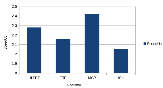
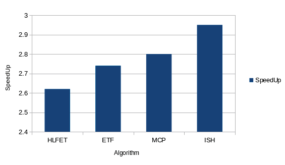
| When the tasks are 35, The MCP algorithm yields | |||||
| highest Speedup value and ISH gives lowest | |||||
| speedup. | |||||
| VI. | Conclusion and Future Scope | ||||
| After Comparative analysis following results | |||||
| were derived: | |||||
| D D D D ) A | |||||
| ( | |||||
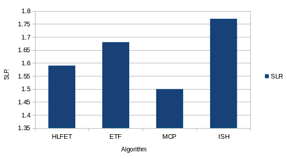
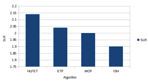
| With 35 task nodes, the MCP algorithm gives lowest | |||||
| SLR value with ISH algorithm giving highest SLR | |||||
| value. | |||||
| With 50 tasks, the ISH shows the lowest SLR value | |||||
| and HLFET gives highest SLR value. | |||||
| With 65 tasks, the ISH has the lesser SLR values | |||||
| and ETF gives highest value. | |||||
| d) Average Speedup: Higher the value of Speedup, | |||||
| more efficient is the algorithm. Fig. 21 shows the | |||||
| Speedup of the all 4 algorithms with various nodes | |||||
| cases. | |||||