1. Introduction
he term texture is somewhat misleading term in computer vision and there is no common or unique definition for texture. Many researchers defined textures based on their specific application. Initially the word texture is taken from textiles. In textures the term texture refers to the weave of various threads tight or loose, even or mixed [2]. The texture provides structural information based on region discrimination shape, surface orientation and spatial arrangement of the object considered [3,4,5,6]. Classification refers; the way different textures or images differ with textural properties or primitives. These textural properties can be statistical, structural and combination of both. One of the oldest, popular and still considered as the bench mark method for classification of textures is the Gray Level Co-occurrence Matrix (GLCM) [7].
The GLCM computes the relative grey level frequencies among the adjacent pair of pixels. Today mostly the GLCM is combined with other methods and it is rarely used individually [8,9,10]. Signal processing methods based on wavelets [11,12,13] and curvelet transforms [14,15] are also widely used for texture classification. The present paper derived a classification method on the wavelet transforms using morphological gradient on the shape descriptors derived on the cross diagonal texture unit. The rest of the paper is organized as below. The section two and three describes the basic concepts of wavelets and morphology. The section four describes the proposed method. The section five and six describes the results and discussions followed by conclusions.
2. II.
3. Basic Concepts of Wavelets
Today the methods based on the Discrete wavelet transform (DWT) are efficiently and successfully used in many scientific fields such as pattern recognition, signal processing, image segmentation, image compression, computer vision, video processing, texture classification and recognition [16,17]. Many research scholars showed significant interest in DWT transform based methods due to its ability to display image at different resolutions and to achieve higher compression ratio.
An image signal can be analyzed by passing it through an analysis filter bank followed by a decimation operation in the wavelet transforms [18,19]. At each decomposition stage the analysis filter bank consists of a low pass and a high pass filter. When the signal goes through these filters it divides into two bands. The averaging operation is known as the low pass filter, extracts the coarse information of a signal. The detail information of the signal is achieved by the high pass filter, which corresponds to a differencing operation. The output of the filtering operations is then decimated by two [20,21].
By performing two separate one-dimensional transforms one can accomplish a two-dimensional transform. For this Firstly, the image is filtered along the x-dimension using low pass and high pass analysis filters and decimated by two. On the left part of the matrix Low pass filtered coefficients are stored and on the right part of the matrix the high pass filtered coefficients are stored. Because of decimation the total size of the transformed image is same as the original image, which is shown in Fig. 1. Then, it is followed by filtering the sub image along the y-dimension and decimated by two. Finally, the image splits into four bands denoted by low-low (LL), high-low (HL), low-high (LH) and high-high (HH) after one-level decomposition as depicted in Fig. 2. III.
4. Basic Concepts of Morphology
One of the well defined non-linear theories of image processing is mathematical morphology [19,22]. Mathematical morphology defines shape and form of the object and it is basically known for its geometry oriented nature. That's why mathematical morphology provides a basic frame work for effective analysis of the object shape features such as size, connectivity and orientation. These features are not easily derived by linear approaches. Mathematical morphology can be applied to binary or gray level images. The morphological operations plays a vital role in boundary and edge detection, noise removal, image enhancement, pre-processing, segmentation, in medical image processing for finding abnormalities and size and volume of the tissues etc. The main advantage of mathematical morphology is all its operations are defined over two simple operations i.e. dilation and erosion.
The fundamental or basic step in morphology is to compare the given objects to be analyzed, classified, pre-processed etc. with an object of known shape termed as a Structuring Element (SE). The image transformation will be resulted in morphology by comparing the object under study (analogous to universe) with a defined shape or SE. The shape of the defined SE element plays a crucial role in morphological processing.
Two basic morphological operations -erosion and dilation are based on Minkowski operations as given in equation ( 1) and ( 2)
X ? B = y?B ? X y(1)X ? B = y?B ? X y(2)Where:
X y = { x + y ? x ? X } (3) B ? = { b ? ?b ? B }(4)B and B ? are Structuring elements Dilation in general makes objects to grow or dilate in size. Erosion makes objects to shrink. The amount and the way that they expand or shrink depend upon the selection of the structuring element. Dilating or eroding without the knowledge of structural element makes no more sense than trying to low pass filter an image without specifying the filter.
Dilation grows or dilates or closes the gaps. Erosion in general shrinks or widens the gaps. The amount and the way they expand or shrink and closes and widens gaps depends upon the selected SE. Dilating or eroding without the knowledge of SE makes no sense than trying to low-pass filter an image without specifying the filter.
Another important pair of morphological operations are closing and opening. They are defined in terms of dilation and erosion, by equations ( 5) and ( 6) respectively
X ? B= ( X ? B) ? B (5) X ? B= ( X ? B ) ? B(6)Dilation followed by erosion is known as closing. Closing connects the objects that are close to each other, fills up small gaps and smoothes the outline of the object by filling up narrow holes. Opening is nothing but erosion followed by dilation. Opening widens small holes and smoothes the objects. Opening operation decreases the size of bright, small details with no prominent effect on the darker gray levels.
Morphological gradient is derived in the present study by evaluating the difference between Dilation and erosion over a 3 x 3 neighborhood. The present paper converted the color is images using RGB quantization process by using 7-bit binary code of 128 colors.
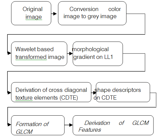
5. a) Derivation of Wavelet based Morphological Gradient Binary Cross Diagonal Shape Descriptors Texture Matrix (WMG-BCDSDTM)
The Texture Unit (TU) and Texture Spectrum (TS) approach was introduced by Wang and He [20]. The TU approach played a significant role in texture analysis, segmentation and classification. The frequency of occurrences of TU in an image is called Texture Spectrum (TS). Several textural features are derived using TS for wide range of applications [4].
In the literature most of the texture analysis methods using texture units based on 3x3 neighboring pixels obtained the texture information by forming a relationship between the center pixel and neighboring pixels. One disadvantage of this approach is they lead to a huge number of texture units 0 to 38-1 if ternary values are considered otherwise 0 to 28-1 texture units if binary values are considered. To overcome this Cross Diagonal Texture Unit (CDTU) is proposed in the literature [1]. Based on the CDTU values Cross diagonal texture matrix (CDTM) is computed [1]. On the CDTM the GLCM features are evaluated for efficient classification [1].
In the CDTM approach the 8neighboring pixels of a 3x3 window are divided into two sets called diagonal and cross Texture Unit Elements (TUE). Each TUE set contains four pixels. The typical dimension of CDTM is 80 x 80. To reduce this dimension CDTU is evaluated using binary representation instead of ternary. In this the Binary CDTM (BCDTM) contains a dimension of 16 x 16. The elements CDTM and BCDTM can be ordered into 16 different ways [1]. To overcome
6. Representation of Representation of BDTUE in the form BCTUE in the form 2x2.Evaluation 2x2.Evaluation of SD Of SD Index(Triangle=4)
Index (Line =2) The advantage of shape descriptors is they don't depend on relative order of texture unit weights. The TU weights can be given in any of the four forms as shown in Fig. 6. The relative TU will change, but shape remains the same. This section presents shape descriptors and also the indexes that are given to shape descriptors. In the proposed Shape Descriptors (SD) the TU weights can be taken in any order. It results the same shape.
2 0 2 1 2 3 2 0 2 2 2 3 2 1 2 2 2 3 2 2 2 2 2 1 2 1 2 0 2 0 2 3Hole shape (Index 0): The all zero's on a 2x2 grid represents a hole shape as shown in the Fig. 7. It gives a TU as zero. 0 0 0 0 Figure7 : Hole shape on 2x2 grid with index value 0 Dot shape (Index 1): The TU with 1, 2, 4 and 8 represents a dot shape. The dot shape will have only a single one as shown in Fig. 8.
1 0 0 1 0 0 0 0 0 0 0 0 0 1 1 0Figure 8 : The four dot shapes on a 2x2 grid with index value 1
1 1 0 1 1 0 1 1 0 1 1 1 1 1 1 0Figure 11 : Representation of triangle shape on a 2x2 grid with index 4 Blob shape (Index 5) : All one's in a 2x2 grid represents a blob shape with TU 15. This is shown in Fig. 12.
1 1 1 1
Figure 12 : Representation of blob shape on a 2x2 grid with index 5
The detailed formation process of Wavelet based Morphological Gradient Binary Cross Diagonal Shape Descriptor Texture Matrix (WMG-BCDSDTM) is shown in Fig. 5. There are only six shape descriptors (0 to 5) on a 2x2 image. Therefore the WMG-BCDSDTM dimension is reduced to 6x6. On this WMG-BCDSDTM the GLCM feature parameters like contrast, correlation, energy and homogeneity are evaluated as given in equation 11, 12, 13 and 14. Horizontal or Vertical line shape (Index 2): The TU 3, 6, 9 and 12 represents a horizontal or vertical line. They contain two adjacent ones as shown in Fig. 9.
???????????? = ? ????? (?? ???? ) 2(11)???1 ??,?? =0 ???????????????? = ? ?? ???? ???1 ??,?? =0 (?? ? ??) 2(12)1 1 0 1 0 0 1 0 0 0 0 1 1 1 1 0Figure 9 : Representation of horizontal and vertical lines on a 2x2 grid with index 2 Diagonal Line shape (Index 3): The other two adjacent one's with TU values 5 and 10 represents diagonal lines as shown in Fig. 10.
0 1 1 0 1 0 0 1Figure 10 : Representation of diagonal line on a 2x2 grid with index 3
0 1 2 3 4 5 0 1 2 3 4 X 5Triangle shape (Index 4) : The three adjacent one's with TU values 7, 11, 13 and 14 represents triangle shape as shown in Fig. 11.
Ho???????????????? = ? ?? ???? 1+(????? ) 2 ???1 ??,?? =0 (13) ?????????????????????? = ? ?? ???? ???1 ??,?? =0 (????? )(?? ??? ) ?? 2(14)Where P ij is the pixel value of the image at position (i, j), µ is mean and ? is standard deviation.
7. V.
8. Results and Discussions
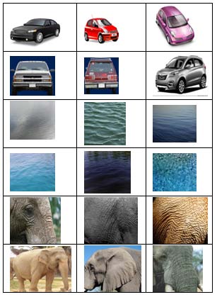
To test the efficiency of the proposed method the present paper evaluated above GLCM features for Water and Elephant images collected from Google database with a resolution of 256x256. The images are as shown in Fig. 13.
9. Conclusion
The proposed Wavelet based Morphological Gradient BCDSDTM is based on CDTM. It reduced the overall dimension of the proposed texture matrix from 81x81 as in the case of CDTM and 16x16 as in the case of Binary CDTM into 6x6. Thus it has reduced lot of complexity. Another disadvantage of the CDTM and BCDTM is it forms 16 different CDTM's for the same texture. The proposed WMG-BCDSDTM overcomes this by representing the four texture elements in the form of a 2x2 grid and deriving shape descriptors on them. The morphological gradient of the present method preserves the shape and boundaries. The proposed WMG-BCDSDTM proves that the WMG-BCDSDTM can be used effectively in wavelet domain and it reduces lot of complexity. The proposed method can also be used in image retrieval system.

| Year 2014 |
| G |
| Average | Average | Average | Average | |
| contrast | correlation | energy | homogeniety | |
| C_1 | 76237.0 | -0.047 | 0.165 | 0.433 |
| C_2 | 52556.8 | -0.051 | 0.164 | 0.422 |
| C_3 107235.9 | -0.038 | 0.166 | 0.462 | |
| C_4 77115.16 | 0.047 | 0.165 | 0.432 | |
| C_5 69522.79 | -0.062 | 0.165 | 0.413 | |
| C_6 70546.15 | -0.047 | 0.182 | 0.444 | |
| C_7 42989.83 | -0.056 | 0.165 | 0.413 | |
| C_8 44555.19 | -0.069 | 0.166 | 0.415 | |
| C_9 55080.92 | -0.054 | 0.164 | 0.415 | |
| C_10 78811.38 | -0.016 | 0.165 | 0.403 | |
| else if ( (contrast > 45000 && contrast <=150000) && |
| homogeneity==0.4 ) |
| print(" Car Texture "); |
| End |
| Based on the |
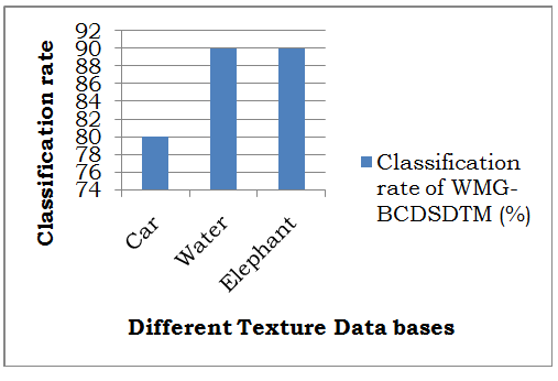
| Texture Database | Classification rate of WMG-BCDSDTM (%) |
| Car | 80 |
| Water | 90 |
| Elephant | 90 |
| Average Classification rate | 86.6 |