1. INTRODUCTION
he compression of an image is very useful in many important areas such as data storage, communication, computation purpose and neural network purpose. The neural networks are being well developed in software computing process. Noise suppression, transform extraction, Parallelism and optimized approximations are some main reasons that useful to artificial neural network for image compression method. The activities of image compression on neural networks implemented in Multi-Layer Perceptron (MLP) [2][3][4][5][6][7][8][9][10][11][12][13], learning vector quantization (LVQ), [14], Self-Organizing Map(SOM),Learning Vector quantization (LVQ) [15,16]. From these network methods, the Back propagation neural network is used for MLP process. In artificial neural network (ANN) uses, Back-Propagation algorithm processed in image compression method [3].The experts used a three-layer BPNN method for compression. The image is used for compression, it is divided into blocks and taken to input neurons, the neurons of input are compressed are taken at output of the hidden layer and the de-compressed images are stored in the output of the hidden layer. This process was implemented in the NCUBE parallel computer and the simulation results produced from network taken a poor image quality in 4:1 compression ratio [3]. By using single network for compression of an image, the result produced from a single network one simple BPNN are poor one. The researches try to increase the performance of an image in neural-network based compression technique. The compress/decompress (CODEC) image blocks are used on various methods for different image blocks regarding to the complexity of blocks. The results produced from image compression are good with neural networks. The cluster of an image blocks into some basic classes based on a complexity measure called activity. The researchers used four BPNNs with different compression rates for each class with neural network. It produces more benefit improvement over basic BPNN. The adaptive approach with proposed the use of complexity measure with block orientation by six BPNNs has given better visual quality [11]. The BPNNs were used for compressing image blocks, after that each pixel in a block was subtracted from the mean value of the block. This method gives some Best-SNR method is used to select the network that gives the best SNR for the block of an image. The overlapping of image blocks in a particular area is used in order to reduce the chess-board effect in de-compressed image. The Best-SNR methods in PSNR produce the visual quality of reconstructed image compared to standard images in JPEG coding. This paper is taken as follows. In section II we discuss multi-layer neural network for image compression. Section III describes the Modified-Levenberg method used in this paper. In section IV, the experimental results of our implementations are taken and discussed and finally in section V we conclude this research and give a summary on it.
2. II.
3. IMAGE COMPRESSION USED WITH MULTI-LAYER NEURAL NETWORKS
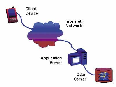
The image compression used with Backpropagation algorithm in multi-layer neural network. The multi-layer neural network is given in Fig. 1. It taken the network with three layers, input, hidden and output layer. Both the input and output layers have the same number of neurons, N. The input and output are connected to each network; the compression can be done with the value of the neurons at the hidden layer. In compression methods, the input image is divided into blocks, for example with 8×8 , 4× 4 or 16 ×16 pixels the block sizes of neurons in the input/output layers which convert to a column vector and fed to the input layer of network; one neuron per pixel. With this basic MLP neural network, compression is conducted in training and application phases as follow.
4. 1) Training
In image compression, the image samples are used to train each network with the back propagation learning rule. In network, the output layer of network will be equal to the input pattern with each layer in a narrow channel. The normalized gray level range, training samples of blocks are converted into vectors. In compression and de-compression can be given in the following equations.
= (1) = (2)In the above equations, f and g are the activation functions which can be linear or nonlinear. ij V and ji W represent the weights of compressor and decompress or, respectively. The extracted N × K transform matrix in compressor and K × N indecompressor of linear neural network are in PCA transform. It minimizes the mean square error between original and reconstructed image. The new spaces are decorrelated led to better compression. For datadependent transform by using linear and nonlinear activation functions in this network results linear and non-linear PCA respectively. In training process of the neural network structure in Fig. 1 is iterative and stopped when the weights convert to their true values. In real applications the training is stopped when the error of equation ( 3) reaches to a threshold or maximum number of iterations limits the iterative process.
(3)
5. 2) Application
When training process is completed and the coupling weights are corrected and the test image is fed into the network and compressed image is obtained in the outputs of hidden layer. The outputs must be applied to the correct number of bits. The same number of total bits is used to represent input and hidden neurons, and then the Compression Ratio (CR) will be the ratio of number of input to hidden neurons. For example, to compress an image block of 8×8, 64 input and output neurons are required. In this case, if the number of hidden neurons is 16 (i.e. block image of size 4× 4), the compression ratio would be 64:16=4:1. But for the same network, if 32 bits floating point is used for coding the compressed image, then the compression ratio will be 1:1, which indicates no compression has occurred. In general, the compression ratio of the basic network is illustrated in Fig ( 1) for an image with n blocks is computed as Eq. ( 4). When training with the LM method, the increment of weights Î?"w can be obtained as follows:
(5)
Where J is the Jacobian matrix, ? is the learning rate which is to be updated using the ? depending on the outcome. In particular, ? is multiplied by decay rate ? (0<?<1) whenever F(w) decreases, whereas ? is divided by ? whenever F(w) increases in a new step.
In de-compressor, the compressed image is converted to a version similar to original image by applying the hidden to output layer de-compression weights on outputs of hidden layer. The outputs of output neurons must be scaled back to the original grayscale range, i.e.[0~255] for 8 bit pixels.
6. 3) Adaptive Approach
The neural network for image compression provides an value for PCA transform. The structure tries to implement the input samples of pixels in the network ©2011 Global Journals Inc. (US) data compression. This is not used in many real applications. This is the main reason that PCA is replaced with its nearest approximate, the dataindependent Discrete Cosine Transform (DCT) transform in real applications. One method for improving the performance of this simple structure is the adaptive approach which uses different networks to compress blocks of the image [2,[5][6][7][8][9][10][11]. The networks have identical structure, but they have different number of neurons in hidden layers, which will result in different compression ratios.
Considering the network of Fig. 1 as the basic structure, we can present the adaptive method as in Fig. 2. In each block is estimated by means of a value to a complexity measure like average of the gray-levels in image block or some other methods. Then for complexity value, one of the available networks is selected and used by Back-propagation algorithm. The code should be transmitted or be saved along the compressed image. In de-compressor or transmitted code along with the compressed image is extracted from the corresponding network. In adaptive approach, the M different networks with k1 -kM neurons in hidden layer. The image with n blocks each having N pixels, the compression ratio is as equation ( 5) that is obtained by modifying equation (4).
7. III. EXISTING LEVENBERG-MARQUARDT THODS
The standard LM training process can be illustrated in the following pseudo-codes, 1. Initialize the weights and parameter ?0 (?=.01 is appropriate). 2. Compute the sum of the squared errors over all inputs F(w) . To consider performance of index is F(w) = eT e using the Newton method. STEP 1: J (w) is called the Jacobian matrix. STEP 2: Next to find the Hessian matrix in k, j elements of the Hessian matrix. STEP 3: The eigenvectors of G are the same as the eigenvectors of H, and the eigen values of G are (?i+?). STEP 4: The matrix G is positive definite by increasing ? until (?i+?)>0 for all i therefore the matrix will be invertible it leads to Levenberg-Marquardt algorithm. STEP 5: For learning parameter, ? is illustrator of steps of actual output movement to desired output. In the standard LM method, ? is a constant number. This paper modifies LM method using ? as: ? = 0.01eT e Where e is a k ×1 matrix therefore eTe is a 1 × 1 therefore [JTJ+?I] is invertible.
For actual output is taken for desired output or errors. The measurement of error is small then, actual output approaches to desired output with soft steps. Therefore error oscillation reduces.
IV.
8. RESULTS AND DISCUSSION
9. CONCLUSION
A picture can say more than a thousand words. However, storing an image can cost more than a million words. This is not always a problem because now computers are capable enough to handle large amounts of data. However, it is often desirable to use the limited resources more efficiently. For instance, digital cameras often have a totally unsatisfactory amount of memory and the internet can be very slow. In these cases, the importance of the compression of image is greatly felt. The rapid increase in the range and use of electronic imaging justifies attention for systematic design of an image compression system and for providing the image quality needed in different applications. There are for image compression. Image compression using neural network technique is efficient when referring to the literature.
In this thesis the use of Multi

![[w1, w2? wN] consists of all weights of the network, e is the error vector comprising the error for all the training examples.](https://computerresearch.org/index.php/computer/article/download/673/version/100188/1-A-Study-on-Image-Compression-with-Neural-Networks_html/1386/image-3.png)

| BIRD 256 IMAGE SIZE | 21.4117 LEVENBERG-MARQUARDT 152.5243 765.969000 METHOD | 22.8879 LEVENBERGMARQUARDT 108.57 MODIFIED | 550.265000 | |||
| METHOD | ||||||
| IMAGE | PSNR | MSE | TIME(SECONDS) | PSNR | MSE | TIME(SECONDS) |
| LENA | 21.7006 | 161.4895 | 3303.3698 | 22.3675 | 148.7677 | 2169.579000 |
| PEPPER be accepted to obtain better reconstructed image 15.0934 188.6425 3411.375000 | 15.3527 | 172.4312 | 2151.516000 | |||
| BABOON quality. Comparing results with basic BNN algorithm 13.9517 195.6905 3614.437000 | 16.4312 | 123.0598 | 2376.734000 | |||
| CROWD shows better performance for the proposed method 14.3570 301.0073 4065.17200 | 15.7204 | 322.2830 | 2208.1410 | |||
| BIRD both with PSNR measure and visibility quality. 25.8375 54.5497 3112.781000 | 26.0312 | 55.6387 | 2056.3698 | |||