1.
Introduction ncompressed text, graphics, audio and video Data require considerable storage capacity for today's storage technology. Similarly for multimedia communications, data transfer of uncompressed images and video over digital network require very high bandwidth. For example, an uncompressed still image of size 640x480 pixels with 24 bits of color require about 7.37 M bits of storage and an uncompressed full-motion video (30 frames/sec) of 10 sec duration needs 2.21 G bits of storage and a bandwidth of 221 M bits/sec. Even if there is availability of enough storage capacity, it is impossible to transmit large number of images or play video (sequence of images) in real time due to insufficient data transfer rates as well as limited network bandwidths.
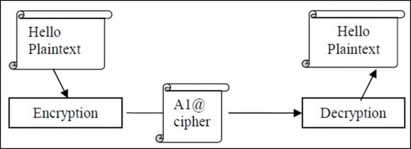
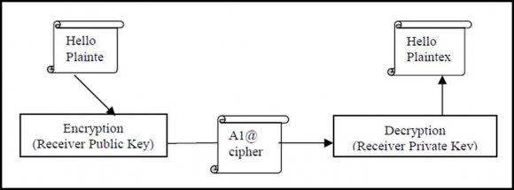
The encryption algorithms aim at achieving confidentiality, not inhibiting unauthorized content duplication. The requirements of these two applications are different. Systems for inhibiting unauthorized content duplication attempt to prevent unauthorized users and devices from getting multimedia data with feasible quality. Such a system could be considered successful if the attacker without the correct key could only get highly degraded contents. Most selective encryption algorithms in the literature are adequate for this purpose. Encryption for confidentiality, on the other hand, must prevent attackers without the correct key from obtaining any intelligible data. Such a system fails if the hacker, after a lot of work, could make out a few words in the encrypted speech or a vague partial image from the encrypted video.
To sum up, at the present state of art technology only solution is to compress Multimedia data before storage and transmission and decompress it at the receiver for play back [1]. Discrete Cosine Transform (DCT) is the Transform of choice in image compression standard such as JPEG. Furthermore DCT has advantages such as simplicity and can be implemented in hardware thereby improving its performance. However, DCT suffer from blocky artifacts around sharp edges at low bit rate.
In general, wavelets in recent years have gained widespread acceptance in signal processing and image compression in particular. Wavelet-based image coders are comprised of three major components: A Wavelet filter bank decomposes the image into wavelet coefficients which are then quantized in a quantizer, finally an entropy encoder encodes these quantized coefficients into an output bit stream (compressed image). Although the interplay among these components is important and one has the freedom to choose each of these components from a pool of candidates, it is often the choice of wavelet filter that is crucial in determining the ultimate performance of the coder.
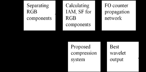
A wide variety of wavelet-based image compression schemes have been developed in recent years [2]. Most of these well known Images coding algorithms use novel quantization and encoding techniques to improve Coding Performance (PSNR). However, they use a fixed wavelet filter built into the algorithm for coding and decoding all types of color images whether it is a natural, synthetic, medical, scanned or compound image. But, in this work we propose dynamic selection of suitable wavelet for different types of images to achieve better PSNR and excellent false acceptance and rejection ratio with minimum computational complexity and better recognition rate.
Wavelets provide new class of powerful algorithm: They can be used for noise reduction, edge detection and compression. The usage of wavelets has superseded the use of DCTs for image compression in JPEG2000 image compression algorithm.
This paper is organized as follows: Importance and procedural steps of wavelet transforms is explained in section II, calculation of statistical parameters like IAM, SF and their importance is explained in section III, Training of counter propagation neural network is presented in section IV, Multilayer feed forward neural network with error back propagation training algorithm is explained in section V, proposed method for dynamic selection of suitable wavelet and effective compression with MLFFNN with EBP and modified RLC is explained in section VI, Simulation results are presented in section VII, Conclusion and future scope is given in section VIII.
2. II.
3. Wavelet Transform of an Image
Wavelet transform is used to decompose an input signal into a series of successive lower resolution reference signals and their associated detail coefficients, which contains the information needed to reconstruct the reference signal at the next higher resolution level.
In discrete wavelet transform, an image signal can be analyzed by passing it through analysis filter bank followed by decimation operation. This analysis filter bank which consists of both low pass and high pass filters at each decomposition stage is commonly used in image compression. When signal passes through these filters, it is split into two bands. The low pass filter, which corresponds to averaging operation, extracts the coarse information of the signal. The high pass filter, which corresponds to differencing operation, extracts the detail information of the signal. The output of the filtering operation is then decimated by two.
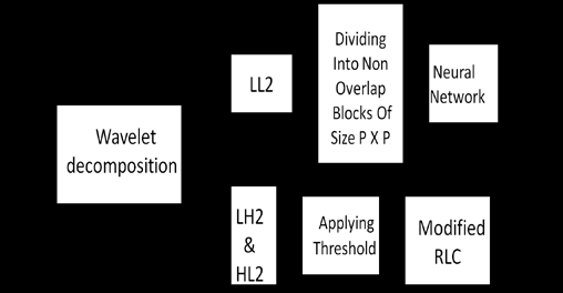
A two dimensional transform can be accomplished by performing two separate one dimensional transform(Fig. 1) First, the image is filtered along the X-dimension using low pass and high pass analysis filter and decimated by two. Low pass filtered coefficients are stored on the left part of the matrix and high pass filtered on the right. Because of decimation, the total size of transformed image is same as the original image. It is then followed by filtering the sub image along the Y-dimension and decimated by two. Finally the image is split into four bands LL1, HL1, LH1 and HH1 through first level decomposition and second stage of filtering. Again the LL1 band is split into four bands viz LL2, HL2, LH2 and HH2 through second level decomposition.
4. Statistical Features of an Image
In literature, many image features have been evaluated: they are range, mean, median, different (mean-median), standard deviation, variance, coefficient variance, skewness, kurtosis, brightness energy [6], gray/colour energy, zero order entropy, first-order entropy and second-order entropy. Other spatial characteristics explored include image gradient [6][7][8][9], spatial frequency (SF) [10] and spectral flatness measure (SFM) [3]. The result shows that almost all the characteristics have no good correlation with the codec performance. However, the image gradient (IAM) and spatial frequency (SF) have strong correlation with the performance of the wavelet-based compression [6][7][8][9]11]. Image gradient measure is a measure of image boundary power and direction. An edge is defined by a change in gray level in gray scale or colour level in colour image. Image gradient is used to provide an indication of activity for an image in terms of edges. Saha and Vemuri [7] defined image gradient as:
? ? ? ? ? ? + ? + + ? = ?? ?? ? = = = ? = 1 1 1 1 1 1 ) 1 , ( ) , ( ) , 1 ( ) , ( * 1 M i N i M i N j j i I j i I j i I j i I N M IAM (1)Where I is intensity value of pixel i, j. The other feature that has strong correlation is the SF in the spatial domain. SF [10] is the mean difference between neighbouring pixels and it specifies the overall image activity. It is defined as:
( ) ( ) ? ? ? ? ? ? ? + ? ? ? ? ? ? ? = ?? ?? ? = ? ? ? = = ? 1 1 2 2 , 1 , 1 1 1 2 1 , , 1 1 M j N k k j k j M j N k k j k j X X MN X X MN SF (2)Where, X is intensity of pixel j, k. Since the result of study shows that there is strong correlation between IAM and SF to the codec performance it is therefore decided to force these features as inputs to the neural network. It is envisaged that these image features are used to select most appropriate wavelet to compress a specific image.
IV.
5. Counter Propagation Neural Network
The counter propagation network is two-layered consisting of two feed forward layers. It performs vector to vector mapping similar to Hetero Associative memory networks. Compared to Bidirectional Associative Memory (BAM), there is no feedback and delay activation during the recall operation mode. The advantage of the Counter propagation network is that it can be trained to perform associative mappings much faster than a typical two-layer network. The counter propagation network is useful in pattern mapping and associations, data compression, and classification.
The network is essentially a partial selforganizing look-up table that maps Rn into Rq and is taught in response to a set of training examples. The objective of the counter propagation network is to map input data vectors Xi into bipolar binary responses Zi, for i=1, 2,?? p. We assume that data vectors can be arranged into p clusters, and the training data are noisy versions of vectors Xi . The essential part of the counter propagation network structure is shown in Fig. 2. However, counter propagation combines two different; novel learning strategies and neither of them is gradient descent technique. The network's recall operation is also different from previously seen architecture.
The first layer of the network is the Kohonen layer, which is trained in the unsupervised winner-takeall mode. Each of the Kohonen layer neurons represents an input cluster or pattern class, so if the layer works in local representation, this particular neurons input and response are larger. Similar input vectors belong to same cluster activate the same m'th neuron of the kohonen layer among all p neurons available in this layer. Note that first-layer neurons are assumed to have continuous activation function during learning. However, during recall they respond with the binary unipolar values 0 and 1, specifically when recalling with input representing a cluster, for example, m and the output vector y of the kohonen layer becomes Such response can be generated as a result of lateral inhibitions within the layer which is to be activated during recall in a physical system. The second layer is called the Grossberg layer due to its outstar learning mode. This layer, with weights Vij functions in a familiar manner
Z=â?"? [Vy](4)With diagonal elements of the operatorâ?"? being a sgn (?) function ope rates component wise on entries of the vector V y. . Let us denote the column vectors of the weight matrix V as v 1 ,v 2 ,?v m ?v p, now each weight vector vm for i=1,2,?p, contains entries that are fanning out from the m' th neuron of the kohonen layer.
6. Substituting (3) & (4) then Z=â?"? [Vm]
(5) Where
V m = [v 1m v 2m ??.v qm ] tIt is observed that the operation of this layer with bipolar binary neurons is simply to output zi=1 if v im >0,and zi=-1 if v im <0, for i=1, 2? q, by assigning any positive and negative values for weights vim highlighted in fig. 2, A desired vector-to-vector mapping x?y?z can be implemented by this architecture. This is done under the assumption that the Kohonen layer responds as expressed in (3). The target vector z for each cluster must be availabe for learning, so that the
V m = z (6)However, this is over simplified weight learning rule for this layer, which is of batch type rather than incremental, it would be appropriate if no statistical relationship exists between input and output vectors within the training pairs(x, z). In practice, such relationships often exist and also needs to establish in the network during training.
The training rule of Kohonen layer involves adjustment of weight vectors in proportion to the probability of occurrence and distribution of winning events. Using the outstar learning rule of eqn (4), incrementally and not binarily as in eqn (6), it permits us to treat a stationary additive noise in output z in a manner similar to the way we considered distributed clusters during the training of the kohonen layer with "noisy" inputs. The outstar learning rule makes use of the fact that the learning of vector pairs , denoted by the set of mappings {(x 1 ,z 1 ),?,(x p, z p )) will be done gradually and thus involve eventual statistical balancing within the weight matrix V. The supervised learning rule for this layer in such a case becomes incremental and takes the form of the out star learning rule.
?V m = ? (z-V m ) (7)Where ? is set to approximately 0.1 at the beginning of learning and reduces gradually during the training process. Index m denotes the number of the winning neurons in the Kohonen layer. Vectors Zi,, i=1, 2 ?p, used for training are stationary random process vectors with statistical properties that make the training possible.
Note that the supervised outstar rule learning eqn (7) starts after completion of the unsupervised training of the first layer. Also as indicated, the weight of the Grossberg layer is adjusted if and only if it fans out from a winning neuron of the kohonen layer. As training progresses, the weights of the second layer tend to converge to the average value of the desired outputs. Let us also note that the unsupervised training of the first layer produces active outputs at indeterminate positions. The second layer introduces ordering in the mapping so that the network becomes a desirable loopup memory table. During the normal recall mode, the grossberg layer output weight values z=vm, connects each output node to the first layer winning neuron. No processing, except for addition and sgn (net) computation, is performed by the output layer neurons if outputs are binary bipolar vectors.
The network discussed and shown in figure 2(a) is simply feed forward and does not refer the counter flow of signals for which the original network was named. The full version of the counter propagation network makes use of bidirectional signal flow. The entire network consists of doubled network from figure 2(a). It can be simultaneously both trained and operated in the recall mode in arrangement as shown in Figure 2(a). This makes possible to use it as an auto associator according to the formula
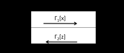
? ?? ? ?? ? ? = ? â?"? 1 [??] â?"? 1 [??] ?(8)Input signals generated by vector x input, and by vector z, desired output, propagate through bidirectional network in opposite directions. Vectors x' and z' are respective outputs that are intended to be approximations, or auto associations, of x and z, respectively.
Let us summarize the main features of this architecture in its simple feed forward version. The counter propagation network functions in the recall mode as the nearest match look-up table. The input vector x finds the weight vector wm which is its closest match among p vectors available in the first layer, then the weights that are entries of vector Vm, which are fanning out from winning mth kohonen's neuron, after sgn (.) computation, become binary outputs. Due to the specific training of the counter propagation network, it outputs the statistical averages of vector z associated with input x. practically, the network performs as well as a look-up table can do to approximate vector matching. Counter propagation can also be used as a continuous function approximator. Assume that the training pairs are (xi, ,zi) and zi =g(xi), where g is a continuous function on the set of input vectors {x}. The mean square error of approximation can be made as small as desired by choosing sufficiently large number p of kohonen layer neurons. However, for continuous function approximation, the network is not as efficient as error back-propagation trained networks, since counter propagation networks can be used for rapid prototyping of mapping and to speed up system development, they typically require orders of magnitude fewer training cycles than usually needed in error back-propagation training.
The counter propagation can use a modified competitive training condition for kohonen layer. Thus it has been assumed that the winning neuron, for which weights are adjusted and one fulfilling condition of yielding the maximum scalar product of the weights and the training pattern vector. Another alternative for training is to choose the winning neuron of the kohonen layer such that the minimum distance criterion is used directly according to the formula
{ } i p i m w x w x ? = ? = ... 2 , 1 min (9)The remaining aspects of weight adaptation and of the training, recall mode. The only difference is that the weights do not have to be renormalized after each step in this training procedure.
7. Multi Layer Feed Forward Neural Network
Consider a feed forward neural network with a single hidden layer denoted by N-h-N, where N is the number of units in the input and output layers, and h is the number of units in the hidden layer. The input layer units are fully connected to the hidden layer units which are in turn fully connected to the output units. The output y, of the jth unit is given by
j N i ji j b i W f Y + = ? =1 (10) k j h j kj k b y W f O + = ? =1(11)Where, in equation ( 10), Wji is the synaptic weight connecting the ith input node to the jth hidden layer, b, is the bias of the ith unit, N is the number of input nodes, f is the activation function, Y, is the output of the hidden layer. Analogously, eqn (11) describes the subsequent layer where Ok is the kth output in the second layer. The networks are trained using the variation of the Back propagation learning algorithm that minimizes the error between network's output and the desired output. This error is given as follows.
( )
? = ? = N k k k d o E 1 (12)Where o and d are the present output and desired outputs of the kth unit of the output layer. For image compression, the number of units in the hidden layer h should be smaller than that in the input and output layers (i.e. h<N). The compressed image is the output of hidden units and is of dimension h.
8. a) Image compression using MLNN
The system for image compression uses two multilayer neural networks. Both networks have N units in the input and output layers, h1 (and h2) units in the hidden layers.
9. i. Training phase
Fig. 3 depicts the system during the training phase, Network-1 is trained to compress and decompress the image (i.e., it is trained to minimize the error between input image and the network output). Then the error is supplied to the second network (Network-2) which is trained to produce the output that is same as its input.
This means that Network-1 is trained to compress and decompress the image and Network-2 is trained to compress and decompress the residual error of Network-1.
Let X1 be the input image of Network-1 and Y1 is its output. The residual error to be minimized by
Network-2 is 1 1 1 X Y E r ? = . The input of Network-2 isgiven by X 2 =X 1 -Y 1 and the residual error is given by ( )
1 1 2 2 Y X Y E r ? ? =. Both networks are trained to perform an identity mapping using error back propagation training algorithm. The compressed coded image is given by C-image= [C1, C2]
Where, vectors C1 and C2 are the outputs for the hidden layer of Network-1 and Network-2. The compression ratio is defined by
2 1 h h N CR + = (13)Where N is the dimension of the image, h1 and h2 are the number of hidden units in Network-1 and Network-2, respectively. The dimension of the compressed image C is h1+h2.
As in Fig ( 3), the Coder-1 (respectively Coder-2) compresses the input of Network-1(respectively Network-2), and Decoder-1(respectively Decoder-2) decompresses the output of the hidden layer of Network-1(respectively Network-2).
Moreover, the input of Network-2 is the residual error between the reconstructed image and original image. During the simulation, it is found that the error is maximal on the edges of the image and this error has to be compressed in a different way when compared to original images. 5. Individual RGB are decomposed into two levels using selected wavelet. 6. Discarding sub bands LH1, HL1, and HH1 of first level and HH2 of second level. Dividing LL2-sub band into non overlapping sub blocks of size P x P. 7. Applying hard threshold to LH2 & HL2-sub bands to discard insignificant coefficients. Encode the threshold coefficients using modified run length coding. 8. Sub blocks of LL1-sub band is given as input to neural network for training. 9. Weight matrix between hidden and output layers, hidden layer output and Modified run length encoded sequence are meant for storage or transmission. b) Algorithm for modified run length coding i. Encoding 1. Read the input vector a (i) and convert it into a single row. 2. Separate the non zero values of input vector a(i), and these non zero values are placed in b(i) . 3. Replace the positions of non zero values with 1's in a (i). 4. Apply run length encoding to a (i). 5. Second part of encoded a (i) and b (i) has to be transmitted.
ii. Decoding: 1. Read the encoded a (i) and b (i).
2. Generate sequence (010101/101010) of size a(i) and concatenate with a(i) 3. Decode vector a(i) and 4. Replace the positions of 1's in vector a (i) with non zero elements from b (i) and reorder the vector a (i).
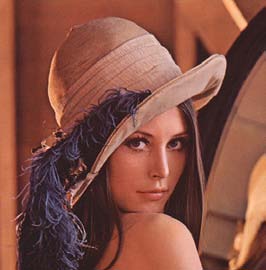
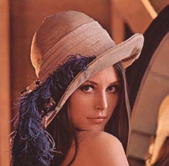
In this proposed method, different types of images of size 512 x 512 pixels are used and grouped into natural like, animal, flower and plants, satellite, people, space/telescope etc. and synthetic like, Cartoon and computer generated images etc, these are taken arbitrarily from many sources. The proposed algorithm is implemented using MATLAB. The PSNR (peak signal to noise ratio) based on MSE (mean square error) is used as a measure of "quality", MSE and PSNR are calculated by the following relations:
( )
1 2 1 1 , , ?? = = ? = M i N j j i j i y x MXN MSE ( ) ? ? ? ? ? ? = MSE PSNR 2 10 255 log 10(15)Where M x N is the image size, x i,j is the input image and yi,j is the reconstructed image. MSE and PSNR are inversely proportional to each other and high [14] with existing lossless and lossy compression methods (fig. 8). Performance of proposed compression system is varied by varying block size and threshold which is given in table4. Here the highest compression (191.53) with better visual quality, PSNR (78.38) and MSE (0.00094) are obtained. In SOFM, compression ratio, reconstructed image quality is poor. SPIHT and embedded zero wavelet (EZW) gives an acceptable visual quality but with poor compression ratio, and computationally expensive.
All these calculations are made based on single neural network of Fig. 3, because no much of difference in quality, MSE, PSNR etc is observed. By using single neural network, training time is reduced dramatically and compression ratio is increased by many folds. Hence it is concluded that only one network is sufficient (fig. 3).
Modified run length encoder's first part of the output sequence is 0101010101/101010??.Hence, it is not required to transmit because, same sequence can be generated at the receiver. However care must be taken for initial synchronization.
10. Different
11. Conclusion and Future Scope
In this paper a novel approach is proposed for dynamic selection of suitable wavelet for a given image under compression.

![y 2 ?..y m .......y p ] = [0 0 ?1 ??0]](https://computerresearch.org/index.php/computer/article/download/89/version/100814/2-Dynamic-Selection-of-Suitable_html/13881/image-3.png)

![Figure 5 : The image decompressor/decoder system. The recovered image is obtained by decoding C= [C1, C2].](https://computerresearch.org/index.php/computer/article/download/89/version/100814/2-Dynamic-Selection-of-Suitable_html/13887/image-9.png)

| VII. Simulation Results and Discussions | |
| (14) | Year 2014 |
| 13 | |
| value of PSNR guarantees Good image quality. Mean square error (MSE), visual quality, Compression ratio and PSNR of different images are calculated and compared | Volume XIV Issue II Version I |
| D D D D D D D D ) F | |
| ( | |
| Procedural steps for modified run length coding Encoding % separating non zero values in vector a % b=[]; % null matrix % for i=1:length(a) % length of a % if abs(a(i))>0 % Identifying non zero values of a % b=[b a(i)]; % storing non zeros values in b % % replacing non zero values in vector a with 1's% for i=1: length(a) % length of a% if abs(a(i))>0 % Identifying non zero values of a% a(i)=1; % replacing 1's % % applying run length encoding % [Enc o/p]=Run length encoder (a) % transmit Enc o/p and non zero values vector b% Decoding % applying run length decoding % %Generate a sequence 010101/1010? of length ( Enc o/p) and concatenate Enc o/p% Seq=0101/1010?.( length ( Enc o/p) | Global Journal of Computer Science and Technology |
| tr=[Seq Enc o/p] | |
| [Dec o/p]= Run length decoder (tr) | |
| %create zero matrix with size Dec o/p vector% | |
| Out= zeros(1, length of Dec o/p) | |
| for i=1:length(Dec o/p) % length of Dec o/p % | |
| if Dec o/p(i)==1 % Identifying 1's Dec o/p % | |
| Out (i) =b (1); % replacing 1's in Dec o/p with | |
| nonzero values in b% | |
| b=b(2: end); %deleting the replaced values% | |
| %out is the decoded vector and it should be reordered to get final | |
| matrix% | |
| © 2014 Global Journals Inc. (US) |
| IAM Red | IAM Green | IAM Blue | SF Red | SF Green | SF Blue | ||||||
| Types Of | Compone | Compone | Compone | Compone | Compone | Compone | |||||
| mages | nt | nt | nt | nt | nt | nt | |||||
| Lena | 12.5292 | 11.8866 | 11.8773 | 15.2399 | 14.5164 | 14.4296 | |||||
| baboon | 40.0599 | 40.3761 | 40.5621 | 39.7834 | 40.0778 | 40.0724 | |||||
| peppersp | 10.3855 | 11.0361 | 10.6255 | 18.3515 | 19.1542 | 16.2229 | |||||
| vis | 26.5328 | 26.6162 | 26.3941 | 38.9153 | 39.1407 | 37.8931 | |||||
| christmas | 19.7346 | 19.0557 | 18.0339 | 37.6165 | 36.9486 | 34.6220 | |||||
| car | 12.3352 | 7.0442 | 5.7128 | 33.9257 | 18.8259 | 15.7576 | |||||
| Sail boat | 17.9651 | 24.1085 | 21.5772 | 18.1433 | 27.3724 | 26.5447 | |||||
| BIOR6.8 | BIOR5.5 | DB10 | DB9 | SYM8 | SYM7 | COIF5 | Best | Wavelet | |||
| Image | |||||||||||
| (1) | (2) | (3) | (4) | (5) | (6) | (7) | wavelet | code | |||
| Lena | 73.8421 | 73.3174 | 73.5816 | 73.5705 | 73.7944 | 73.7118 | 73.8281 | BIOR6.8 | 1 | ||
| baboon | 65.6505 | 65.6519 | 65.5956 | 65.5566 | 65.5733 | 65.5981 | 65.6155 | BIOR5.5 | 2 | ||
| peppersp | 73.3050 | 72.5798 | 73.2225 | 72.4431 | 72.6919 | 73.5854 | 73.1407 | SYM7 | 6 | ||
| vis | 66.0113 | 65.7960 | 65.9696 | 65.9763 | 66.0317 | 66.0228 | 65.7798 | SYM8 | 5 | ||
| christmas | 67.6023 | 67.0274 | 67.2650 | 67.2799 | 67.5409 | 67.3391 | 67.6140 | COIF5 | 7 | ||
| car | 73.5311 | 70.9601 | 71.2950 | 71.5879 | 71.4965 | 71.4743 | 71.4929 | DB9 | 4 | ||
| Sail boat | 70.3648 | 69.9146 | 70.4476 | 70.1378 | 70.1823 | 70.4359 | 70.2575 | DB10 | 3 | ||
| Year 2014 | |||||
| 14 | |||||
| Volume XIV Issue II Version I | |||||
| D D D D ) F | |||||
| ( | |||||
| Global Journal of Computer Science and Technology | Block size 7x7 10x10 14x14 | Hard Threshold HL2 LH2 0.2 0.3 0.2 0.45 0.2 0.4 | MSE 0.0027 0.0030 0.0029 | PSNR 73.8421 73.4040 73.5196 | CR 77.6340 121.2133 136.5969 |
| Technique | MSE | PSN | CR |
| R | |||
| Proposed | 0.0029 73.51 | 136.5 | |
| method | 96 | 969 | |
| SPIHT | 25.33 34.09 5.95 | ||
| EZW | 46.11 31.49 3.07 | ||
| SOFM | 73.72 29.45 8.92 | ||
| Block | Hard | ||
| size | Threshold MSE | PSNR CR | |
| HL2 LH2 | |||
| 7x7 | 0.2 0.3 | 0.000864 78.763 102.48 | |
| 10x10 0.2 0.45 0.000964 78.288 164.21 | |||
| 14x14 0.2 0.4 | 0.000944 78.380 191.53 | ||